TrendFriendOverview
TrendFriend (TF) combines various technical analysis components, including trend calculations, moving averages, RSI signals, and Fair Value Gaps (FVG) detection to determine trend reversal and continuation points. The FVG feature identifies potential consolidation periods and displays mitigation levels.
Features
Trend Analysis: Utilizes short and long-term Running Moving Averages (RMA) to identify trends.
Average True Range (ATR): Plots ATR to depict market volatility.
RSI Signals: Calculates RSI and provides buy/sell signals based on RSI conditions.
Fair Value Gaps (FVG): Detects FVG patterns and offers options for customization, including dynamic FVG, mitigation levels, and auto threshold.
Usage
Buy Signals: Generated based on pullback conditions, contra-buy signals, and crossovers of specified moving averages.
Sell Signals: Generated based on pullback conditions, contra-sell signals, and crossunders of specified moving averages.
Visualization: FVG areas are visually represented on the chart, and unmitigated levels can be displayed.
Configuration
Adjustable parameters for trend periods, ATR length, RSI settings, FVG threshold, and display preferences.
Dynamic FVG detection and mitigation level visualization can be enabled/disabled.
Usage Example
Trend Analysis: Identify trends with short and long-term moving averages.
RSI Signals: Interpret RSI signals for potential reversals.
FVG Detection: Visualize Fair Value Gaps and mitigation levels on the chart.
Buy/Sell Signals: Receive alerts for buy/sell signals based on specified conditions.
Disclaimer
This Pine Script code is subject to the terms of the Mozilla Public License 2.0. Use this code at your own risk, and always conduct additional analysis before making trading decisions.
Author
Author: devoperator84
License: Mozilla Public License 2.0
Buscar en scripts para "moving averages"
RAINBOW AVERAGES - INDICATOR - (AS) - 1/3
-INTRODUCTION:
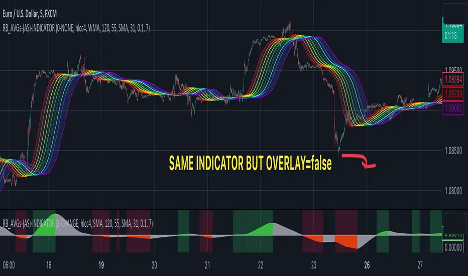
This is the first of three scripts I intend to publish using rainbow indicators. This script serves as a groundwork for the other two. It is a RAINBOW MOVING AVERAGES indicator primarily designed for trend detection. The upcoming script will also be an indicator but with overlay=false (below the chart, not on it) and will utilize RAINBOW BANDS and RAINBOW OSCILLATOR. The third script will be a strategy combining all of them.
RAINBOW moving averages can be used in various ways, but this script is mainly intended for trend analysis. It is meant to be used with overlay=true, but if the user wishes, it can be viewed below the chart. To achieve this, you need to change the code from overlay=true to false and turn off the first switch that plots the rainbow on the chart (or simply move the indicator to a new pane below). By doing this, you will be able to see how all four conditions used to detect trends work on the chart. But let's not get ahead of ourselves.
-WHAT IS IT:
In its simplest form, this indicator uses 10 moving averages colored like a rainbow. The calculation is as follows:
MA0: This is the main moving average and can be defined with the type (SMA, EMA, RMA, WMA, SINE), length, and price source. However, the second moving average (MA1) is calculated using MA0 as its source, MA2 uses MA1 as the data source, and so on, until the last one, MA9. Hence, there are 10 moving averages. The first moving average is special as all the others derive from it. This indicator has many potential uses, such as entry/exit signals, volatility indication, and stop-loss placement, but for now, we will focus on trend detection.
-TREND DETECTION:
The indicator offers four different background color options based on the user's preference:
0-NONE: No background color is applied as no trend detection tools is being used (boring)
1-CHANGE: The background color is determined by summing the changes of all 10 moving averages (from two bars). If the sum is positive and not falling, the background color is GREEN. If the sum is negative and not rising, the background color is RED. From early testing, it works well for the beginning of a movement but not so much for a lasting trend.
2-RAINBW: The background color is green when all the moving averages are in ascending order, indicating a bullish trend. It is red when all the moving averages are in descending order, indicating a bearish trend. For example, if MA1>MA2>MA3>MA4..., the background color is green. If MA1 threshold, and red indicates width < -threshold.
4-DIRECT: The background color is determined by counting the number of moving averages that are either above or below the input source. If the specified number of moving averages is above the source, the background color is green. If the specified number of moving averages is below the source, the background color is red. If all ten MAs are below the price source, the indicator will show 10, and if all ten MAs are above, it will show -10. The specific value will be set later in the settings (same for 3-TSHOLD variant). This method works well for lasting trends.
Note: If the indicator is turned into a below-chart version, all four color options can be seen as separate indicators.
-PARAMETERS - SETTINGS:
The first line is an on/off switch to plot the skittles indicator (and some info in the tooltip). The second line has already been discussed, which is the background color and the selection of the source (only used for MA0!).
The line "MA1: TYP/LEN" is where we define the parameters of MA0 (important). We choose from the types of moving averages (SMA, EMA, RMA, WMA, SINE) and set the length.
Important Note: It says MA1, but it should be MA0!.
The next line defines whether we want to smooth MA1 (which is actually MA0) and the period for smoothing. When smoothing is turned on, MA0 will be smoothed using a 3-pole super smoother. It's worth noting that although this only applies to MA0, as the other MAs are derived from it, they will also be smoothed.
In the line below, we define the type and length of MAs for MA2 (and other MAs except MA0). The same type and length are used for MA1 to MA9. It's important to remember that these values should be smaller. For example, if we set 55, it means that MA1 is the average of 55 periods of MA0, MA2 will be 55 periods of MA1, and so on. I encourage trying different combinations of MA types as it can be easily adjusted for ur type of trading. RMA looks quirky.
Moving on to the last line, we define some inputs for the background color:
TSH: The threshold value when using 3-TSHOLD-BGC. It's a good idea to change the chart to a pane below for easier adjustment. The default values are based on EURUSD-5M.
BG_DIR: The value that must be crossed or equal to the MA score if using 4-DIRECT-BGC. There are 10 MAs, so the maximum value is also 10. For example, if you set it to 9, it means that at least 9 MAs must be below/above the price for the script to detect a trend. Higher values are recommended as most of the time, this indicator oscillates either around the maximum or minimum value.
-SUMMARY OF SETTINGS:
L1 - PLOT MAs and general info tooltip
L2 - Select the source for MA0 and type of trend detection.
L3 - Set the type and length of MA0 (important).
L4 - Turn smoothing on/off for MA0 and set the period for super smoothing.
L5 - Set the type and length for the rest of the MAs.
L6 - Set values if using 4-DIRECT or 3-TSHOLD for the trend detection.
-OTHERS:
To see trend indicators, you need to turn off the plotting of MAs (first line), and then choose the variant you want for the background color. This will plot it on the chart below.
Keep in mind that M1 int settings stands for MA0 and MA2 for all of the 9 MAs left.
Yes, it may seem more complicated than it actually is. In a nutshell, these are 10 MAs, and each one after MA0 uses the previous one as its source. Plus few conditions for range detection. rest is mainly plots and colors.
There are tooltips to help you with the parameters.
I hope this will be useful to someone. If you have any ideas, feedback, or spot errors in the code, LET ME KNOW.
Stay tuned for the remaining two scripts using skittles indicators and check out my other scripts.
-ALSO:
I'm always looking for ideas for interesting indicators and strategies that I could code, so if you don't know Pinescript, just message me, and I would be glad to write your own indicator/strategy for free, obviously.
-----May the force of the market be with you, and until we meet again,
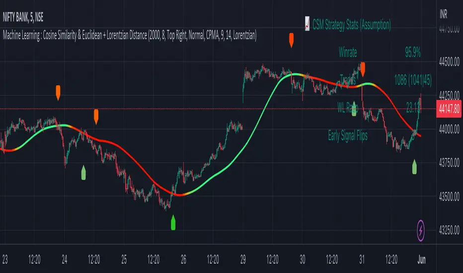
Machine Learning : Cosine Similarity & Euclidean DistanceIntroduction:
This script implements a comprehensive trading strategy that adheres to the established rules and guidelines of housing trading. It leverages advanced machine learning techniques and incorporates customised moving averages, including the Conceptive Price Moving Average (CPMA), to provide accurate signals for informed trading decisions in the housing market. Additionally, signal processing techniques such as Lorentzian, Euclidean distance, Cosine similarity, Know sure thing, Rational Quadratic, and sigmoid transformation are utilised to enhance the signal quality and improve trading accuracy.
Features:
Market Analysis: The script utilizes advanced machine learning methods such as Lorentzian, Euclidean distance, and Cosine similarity to analyse market conditions. These techniques measure the similarity and distance between data points, enabling more precise signal identification and enhancing trading decisions.
Cosine similarity:
Cosine similarity is a measure used to determine the similarity between two vectors, typically in a high-dimensional space. It calculates the cosine of the angle between the vectors, indicating the degree of similarity or dissimilarity.
In the context of trading or signal processing, cosine similarity can be employed to compare the similarity between different data points or signals. The vectors in this case represent the numerical representations of the data points or signals.
Cosine similarity ranges from -1 to 1, with 1 indicating perfect similarity, 0 indicating no similarity, and -1 indicating perfect dissimilarity. A higher cosine similarity value suggests a closer match between the vectors, implying that the signals or data points share similar characteristics.
Lorentzian Classification:
Lorentzian classification is a machine learning algorithm used for classification tasks. It is based on the Lorentzian distance metric, which measures the similarity or dissimilarity between two data points. The Lorentzian distance takes into account the shape of the data distribution and can handle outliers better than other distance metrics.
Euclidean Distance:
Euclidean distance is a distance metric widely used in mathematics and machine learning. It calculates the straight-line distance between two points in Euclidean space. In two-dimensional space, the Euclidean distance between two points (x1, y1) and (x2, y2) is calculated using the formula sqrt((x2 - x1)^2 + (y2 - y1)^2).
Dynamic Time Windows: The script incorporates a dynamic time window function that allows users to define specific time ranges for trading. It checks if the current time falls within the specified window to execute the relevant trading signals.
Custom Moving Averages: The script includes the CPMA, a powerful moving average calculation. Unlike traditional moving averages, the CPMA provides improved support and resistance levels by considering multiple price types and employing a combination of Exponential Moving Averages (EMAs) and Simple Moving Averages (SMAs). Its adaptive nature ensures responsiveness to changes in price trends.
Signal Processing Techniques: The script applies signal processing techniques such as Know sure thing, Rational Quadratic, and sigmoid transformation to enhance the quality of the generated signals. These techniques improve the accuracy and reliability of the trading signals, aiding in making well-informed trading decisions.
Trade Statistics and Metrics: The script provides comprehensive trade statistics and metrics, including total wins, losses, win rate, win-loss ratio, and early signal flips. These metrics offer valuable insights into the performance and effectiveness of the trading strategy.
Usage:
Configuring Time Windows: Users can customize the time windows by specifying the start and finish time ranges according to their trading preferences and local market conditions.
Signal Interpretation: The script generates long and short signals based on the analysis, custom moving averages, and signal processing techniques. Users should pay attention to these signals and take appropriate action, such as entering or exiting trades, depending on their trading strategies.
Trade Statistics: The script continuously tracks and updates trade statistics, providing users with a clear overview of their trading performance. These statistics help users assess the effectiveness of the strategy and make informed decisions.
Conclusion:
With its adherence to housing trading rules, advanced machine learning methods, customized moving averages like the CPMA, and signal processing techniques such as Lorentzian, Euclidean distance, Cosine similarity, Know sure thing, Rational Quadratic, and sigmoid transformation, this script offers users a powerful tool for housing market analysis and trading. By leveraging the provided signals, time windows, and trade statistics, users can enhance their trading strategies and improve their overall trading performance.
Disclaimer:
Please note that while this script incorporates established tradingview housing rules, advanced machine learning techniques, customized moving averages, and signal processing techniques, it should be used for informational purposes only. Users are advised to conduct their own analysis and exercise caution when making trading decisions. The script's performance may vary based on market conditions, user settings, and the accuracy of the machine learning methods and signal processing techniques. The trading platform and developers are not responsible for any financial losses incurred while using this script.
By publishing this script on the platform, traders can benefit from its professional presentation, clear instructions, and the utilisation of advanced machine learning techniques, customised moving averages, and signal processing techniques for enhanced trading signals and accuracy.
I extend my gratitude to TradingView, LUX ALGO, and JDEHORTY for their invaluable contributions to the trading community. Their innovative scripts, meticulous coding patterns, and insightful ideas have profoundly enriched traders' strategies, including my own.
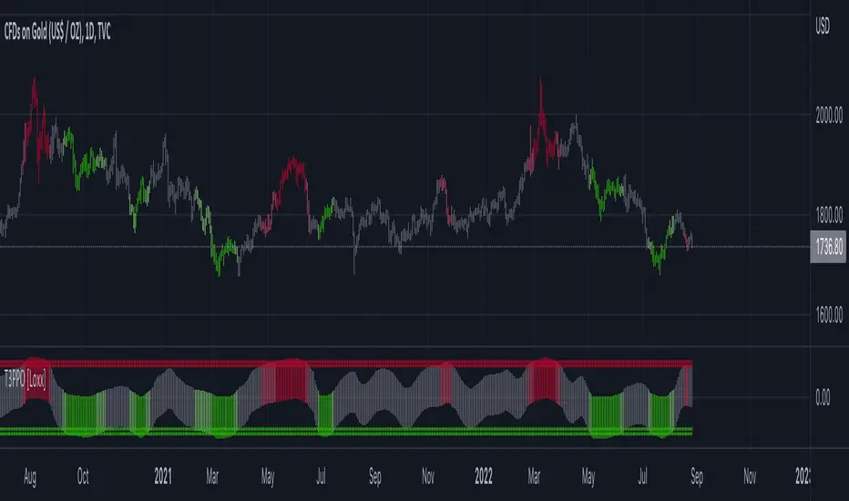
T3 PPO [Loxx]T3 PPO is a percentage price oscillator indicator using T3 moving average. This indicator is used to spot reversals. Dark red is upward price exhaustion, dark green is downward price exhaustion.
What is Percentage Price Oscillator (PPO)?
The percentage price oscillator (PPO) is a technical momentum indicator that shows the relationship between two moving averages in percentage terms. The moving averages are a 26-period and 12-period exponential moving average (EMA).
The PPO is used to compare asset performance and volatility, spot divergence that could lead to price reversals, generate trade signals, and help confirm trend direction.
What is the T3 moving average?
Better Moving Averages Tim Tillson
November 1, 1998
Tim Tillson is a software project manager at Hewlett-Packard, with degrees in Mathematics and Computer Science. He has privately traded options and equities for 15 years.
Introduction
"Digital filtering includes the process of smoothing, predicting, differentiating, integrating, separation of signals, and removal of noise from a signal. Thus many people who do such things are actually using digital filters without realizing that they are; being unacquainted with the theory, they neither understand what they have done nor the possibilities of what they might have done."
This quote from R. W. Hamming applies to the vast majority of indicators in technical analysis . Moving averages, be they simple, weighted, or exponential, are lowpass filters; low frequency components in the signal pass through with little attenuation, while high frequencies are severely reduced.
"Oscillator" type indicators (such as MACD , Momentum, Relative Strength Index ) are another type of digital filter called a differentiator.
Tushar Chande has observed that many popular oscillators are highly correlated, which is sensible because they are trying to measure the rate of change of the underlying time series, i.e., are trying to be the first and second derivatives we all learned about in Calculus.
We use moving averages (lowpass filters) in technical analysis to remove the random noise from a time series, to discern the underlying trend or to determine prices at which we will take action. A perfect moving average would have two attributes:
It would be smooth, not sensitive to random noise in the underlying time series. Another way of saying this is that its derivative would not spuriously alternate between positive and negative values.
It would not lag behind the time series it is computed from. Lag, of course, produces late buy or sell signals that kill profits.
The only way one can compute a perfect moving average is to have knowledge of the future, and if we had that, we would buy one lottery ticket a week rather than trade!
Having said this, we can still improve on the conventional simple, weighted, or exponential moving averages. Here's how:
Two Interesting Moving Averages
We will examine two benchmark moving averages based on Linear Regression analysis.
In both cases, a Linear Regression line of length n is fitted to price data.
I call the first moving average ILRS, which stands for Integral of Linear Regression Slope. One simply integrates the slope of a linear regression line as it is successively fitted in a moving window of length n across the data, with the constant of integration being a simple moving average of the first n points. Put another way, the derivative of ILRS is the linear regression slope. Note that ILRS is not the same as a SMA ( simple moving average ) of length n, which is actually the midpoint of the linear regression line as it moves across the data.
We can measure the lag of moving averages with respect to a linear trend by computing how they behave when the input is a line with unit slope. Both SMA (n) and ILRS(n) have lag of n/2, but ILRS is much smoother than SMA .
Our second benchmark moving average is well known, called EPMA or End Point Moving Average. It is the endpoint of the linear regression line of length n as it is fitted across the data. EPMA hugs the data more closely than a simple or exponential moving average of the same length. The price we pay for this is that it is much noisier (less smooth) than ILRS, and it also has the annoying property that it overshoots the data when linear trends are present.
However, EPMA has a lag of 0 with respect to linear input! This makes sense because a linear regression line will fit linear input perfectly, and the endpoint of the LR line will be on the input line.
These two moving averages frame the tradeoffs that we are facing. On one extreme we have ILRS, which is very smooth and has considerable phase lag. EPMA has 0 phase lag, but is too noisy and overshoots. We would like to construct a better moving average which is as smooth as ILRS, but runs closer to where EPMA lies, without the overshoot.
A easy way to attempt this is to split the difference, i.e. use (ILRS(n)+EPMA(n))/2. This will give us a moving average (call it IE /2) which runs in between the two, has phase lag of n/4 but still inherits considerable noise from EPMA. IE /2 is inspirational, however. Can we build something that is comparable, but smoother? Figure 1 shows ILRS, EPMA, and IE /2.
Filter Techniques
Any thoughtful student of filter theory (or resolute experimenter) will have noticed that you can improve the smoothness of a filter by running it through itself multiple times, at the cost of increasing phase lag.
There is a complementary technique (called twicing by J.W. Tukey) which can be used to improve phase lag. If L stands for the operation of running data through a low pass filter, then twicing can be described by:
L' = L(time series) + L(time series - L(time series))
That is, we add a moving average of the difference between the input and the moving average to the moving average. This is algebraically equivalent to:
2L-L(L)
This is the Double Exponential Moving Average or DEMA , popularized by Patrick Mulloy in TASAC (January/February 1994).
In our taxonomy, DEMA has some phase lag (although it exponentially approaches 0) and is somewhat noisy, comparable to IE /2 indicator.
We will use these two techniques to construct our better moving average, after we explore the first one a little more closely.
Fixing Overshoot
An n-day EMA has smoothing constant alpha=2/(n+1) and a lag of (n-1)/2.
Thus EMA (3) has lag 1, and EMA (11) has lag 5. Figure 2 shows that, if I am willing to incur 5 days of lag, I get a smoother moving average if I run EMA (3) through itself 5 times than if I just take EMA (11) once.
This suggests that if EPMA and DEMA have 0 or low lag, why not run fast versions (eg DEMA (3)) through themselves many times to achieve a smooth result? The problem is that multiple runs though these filters increase their tendency to overshoot the data, giving an unusable result. This is because the amplitude response of DEMA and EPMA is greater than 1 at certain frequencies, giving a gain of much greater than 1 at these frequencies when run though themselves multiple times. Figure 3 shows DEMA (7) and EPMA(7) run through themselves 3 times. DEMA^3 has serious overshoot, and EPMA^3 is terrible.
The solution to the overshoot problem is to recall what we are doing with twicing:
DEMA (n) = EMA (n) + EMA (time series - EMA (n))
The second term is adding, in effect, a smooth version of the derivative to the EMA to achieve DEMA . The derivative term determines how hot the moving average's response to linear trends will be. We need to simply turn down the volume to achieve our basic building block:
EMA (n) + EMA (time series - EMA (n))*.7;
This is algebraically the same as:
EMA (n)*1.7-EMA( EMA (n))*.7;
I have chosen .7 as my volume factor, but the general formula (which I call "Generalized Dema") is:
GD (n,v) = EMA (n)*(1+v)-EMA( EMA (n))*v,
Where v ranges between 0 and 1. When v=0, GD is just an EMA , and when v=1, GD is DEMA . In between, GD is a cooler DEMA . By using a value for v less than 1 (I like .7), we cure the multiple DEMA overshoot problem, at the cost of accepting some additional phase delay. Now we can run GD through itself multiple times to define a new, smoother moving average T3 that does not overshoot the data:
T3(n) = GD ( GD ( GD (n)))
In filter theory parlance, T3 is a six-pole non-linear Kalman filter. Kalman filters are ones which use the error (in this case (time series - EMA (n)) to correct themselves. In Technical Analysis , these are called Adaptive Moving Averages; they track the time series more aggressively when it is making large moves.
Quad MAFor a dive into the fine details, see the source code/documentation.
Quad MA is a program designed to allow a wide range of flexibility in overlaying multiple moving averages onto a chart.
This program handles the ability to:
- Overlay Up to 4 moving averages on the chart.
- Change the length of each moving average.
- Adjust optional values for special moving averages
(least squares and Arnaud Legoux)
- Change the color for each moving average.
- Change the type of each moving average individually.
- Change the visibility of each moving average.
- Change the source of the moving averages.
- Set alerts for a cross between any two moving averages.

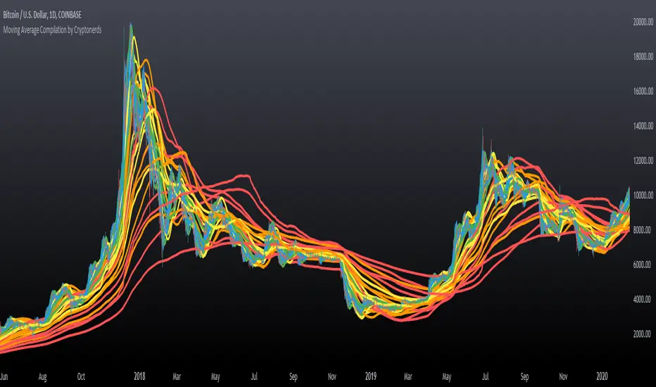
Moving Average Compilation by CryptonerdsThis script contains all commonly used types of moving averages in a single script. To our surprise, it turned out that there was no script available yet that contains multiple types of moving averages.
The following types of moving averages are included:
Simple Moving Averages (SMA)
Exponential Moving Averages (EMA)
Double Exponential Moving Averages (DEMA)
Display Triple Exponential Moving Averages (TEMA)
Display Weighted Moving Averages (WMA)
Display Hull Moving Averages (HMA)
Wilder's exponential moving averages (RMA)
Volume-Weighted Moving Averages (VWMA)
The user can configure what type of moving averages are displayed, including the length and up to five multiple moving averages per type. If you have any other request related to adding moving averages, please leave a comment in the section below.
If you've learned something new and found value, leave us a message to show your support!
Levels Of Interest------------------------------------------------------------------------------------
LEVELS OF INTEREST (LOI)
TRADING INDICATOR GUIDE
------------------------------------------------------------------------------------
Table of Contents:
1. Indicator Overview & Core Functionality
2. VWAP Foundation & Historical Context
3. Multi-Timeframe VWAP Analysis
4. Moving Average Integration System
5. Trend Direction Signal Detection
6. Visual Design & Display Features
7. Custom Level Integration
8. Repaint Protection Technology
9. Practical Trading Applications
10. Setup & Configuration Recommendations
------------------------------------------------------------------------------------
1. INDICATOR OVERVIEW & CORE FUNCTIONALITY
------------------------------------------------------------------------------------
The LOI indicator combines multiple VWAP calculations with moving averages across different timeframes. It's designed to show where institutional money is flowing and help identify key support and resistance levels that actually matter in today's markets.
Primary Functions:
- Multi-timeframe VWAP analysis (Daily, Weekly, Monthly, Yearly)
- Advanced moving average integration (EMA, SMA, HMA)
- Real-time trend direction detection
- Institutional flow analysis
- Dynamic support/resistance identification
Target Users: Day traders, swing traders, position traders, and institutional analysts seeking comprehensive market structure analysis.
------------------------------------------------------------------------------------
2. VWAP FOUNDATION & HISTORICAL CONTEXT
------------------------------------------------------------------------------------
Historical Development: VWAP started in the 1980s when big institutional traders needed a way to measure if they were getting good fills on their massive orders. Unlike regular price averages, VWAP weighs each price by the volume traded at that level. This makes it incredibly useful because it shows you where most of the real money changed hands.
Mathematical Foundation: The basic math is simple: you take each price, multiply it by the volume at that price, add them all up, then divide by total volume. What you get is the true "average" price that reflects actual trading activity, not just random price movements.
Formula: VWAP = Σ(Price × Volume) / Σ(Volume)
Where typical price = (High + Low + Close) / 3
Institutional Behavior Patterns:
- When price trades above VWAP, institutions often look to sell
- When it's below, they're usually buying
- Creates natural support and resistance that you can actually trade against
- Serves as benchmark for execution quality assessment
------------------------------------------------------------------------------------
3. MULTI-TIMEFRAME VWAP ANALYSIS
------------------------------------------------------------------------------------
Core Innovation: Here's where LOI gets interesting. Instead of just showing daily VWAP like most indicators, it displays four different timeframes simultaneously:
**Daily VWAP Implementation**:
- Resets every morning at market open
- Provides clearest picture of intraday institutional sentiment
- Primary tool for day trading strategies
- Most responsive to immediate market conditions
**Weekly VWAP System**:
- Resets each Monday (or first trading day)
- Smooths out daily noise and volatility
- Perfect for swing trades lasting several days to weeks
- Captures weekly institutional positioning
**Monthly VWAP Analysis**:
- Resets at beginning of each calendar month
- Captures bigger institutional rebalancing at month-end
- Fund managers often operate on monthly mandates
- Significant weight in intermediate-term analysis
**Yearly VWAP Perspective**:
- Resets annually for full-year institutional view
- Shows long-term institutional positioning
- Where pension funds and sovereign wealth funds operate
- Critical for major trend identification
Confluence Zone Theory: The magic happens when multiple VWAP levels cluster together. These confluence zones often become major turning points because different types of institutional money all see value at the same price.
------------------------------------------------------------------------------------
4. MOVING AVERAGE INTEGRATION SYSTEM
------------------------------------------------------------------------------------
Multi-Type Implementation: The indicator includes three types of moving averages, each with its own personality and application:
**Exponential Moving Averages (EMAs)**:
- React quickly to recent price changes
- Displayed as solid lines for easy identification
- Optimal performance in trending market conditions
- Higher sensitivity to current price action
**Simple Moving Averages (SMAs)**:
- Treat all historical data points equally
- Appear as dashed lines in visual display
- Slower response but more reliable in choppy conditions
- Traditional approach favored by institutional traders
**Hull Moving Averages (HMAs)**:
- Newest addition to the system (dotted line display)
- Created by Alan Hull in 2005
- Solves classic moving average dilemma: speed vs. accuracy
- Manages to be both responsive and smooth simultaneously
Technical Innovation: Alan Hull's solution addresses the fundamental problem where moving averages are either too slow (missing moves) or too fast (generating false signals). HMAs achieve optimal balance through weighted calculation methodology.
Period Configuration:
- 5-period: Short-term momentum assessment
- 50-period: Intermediate trend identification
- 200-period: Long-term directional confirmation
------------------------------------------------------------------------------------
5. TREND DIRECTION SIGNAL DETECTION
------------------------------------------------------------------------------------
Real-Time Momentum Analysis: One of LOI's best features is its real-time trend detection system. Next to each moving average, visual symbols provide immediate trend assessment:
Symbol System:
- ▲ Rising average (bullish momentum confirmation)
- ▼ Falling average (bearish momentum indication)
- ► Flat average (consolidation or indecision period)
Update Frequency: These signals update in real-time with each new price tick and function across all configured timeframes. Traders can quickly scan daily and weekly trends to assess alignment or conflicting signals.
Multi-Timeframe Trend Analysis:
- Simultaneous daily and weekly trend comparison
- Immediate identification of trend alignment
- Early warning system for potential reversals
- Momentum confirmation for entry decisions
------------------------------------------------------------------------------------
6. VISUAL DESIGN & DISPLAY FEATURES
------------------------------------------------------------------------------------
Color Psychology Framework: The color scheme isn't random but based on psychological associations and trading conventions:
- **Blue Tones**: Institutional neutrality (VWAP levels)
- **Green Spectrum**: Growth and stability (weekly timeframes)
- **Purple Range**: Longer-term sophistication (monthly analysis)
- **Orange Hues**: Importance and attention (yearly perspective)
- **Red Tones**: User-defined significance (custom levels)
Adaptive Display Technology: The indicator automatically adjusts decimal places based on the instrument you're trading. High-priced stocks show 2 decimals, while penny stocks might show 8. This keeps the display incredibly clean regardless of what you're analyzing - no cluttered charts or overwhelming information overload.
Smart Labeling System: Advanced positioning algorithm automatically spaces all elements to prevent overlap, even during extreme zoom levels or multiple timeframe analysis. Every level stays clearly readable without any visual chaos disrupting your analysis.
------------------------------------------------------------------------------------
7. CUSTOM LEVEL INTEGRATION
------------------------------------------------------------------------------------
User-Defined Level System: Beyond the calculated VWAP and moving average levels, traders can add custom horizontal lines at any price point for personalized analysis.
Strategic Applications:
- **Psychological Levels**: Round numbers, previous significant highs/lows
- **Technical Levels**: Fibonacci retracements, pivot points
- **Fundamental Targets**: Analyst price targets, earnings estimates
- **Risk Management**: Stop-loss and take-profit zones
Integration Features:
- Seamless incorporation with smart labeling system
- Custom color selection for visual organization
- Extension capabilities across all chart timeframes
- Maintains display clarity with existing indicators
------------------------------------------------------------------------------------
8. REPAINT PROTECTION TECHNOLOGY
------------------------------------------------------------------------------------
Critical Trading Feature: This addresses one of the most significant issues in live trading applications. Most multi-timeframe indicators "repaint," meaning they display different signals when viewing historical data versus real-time analysis.
Protection Benefits:
- Ensures every displayed signal could have been traded when it appeared
- Eliminates discrepancies between historical and live analysis
- Provides realistic performance expectations
- Maintains signal integrity across chart refreshes
Configuration Options:
- **Protection Enabled**: Default setting for live trading
- **Protection Disabled**: Available for backtesting analysis
- User-selectable toggle based on analysis requirements
- Applies to all multi-timeframe calculations
Implementation Note: With protection enabled, signals may appear one bar later than without protection, but this ensures all signals represent actionable opportunities that could have been executed in real-time market conditions.
------------------------------------------------------------------------------------
9. PRACTICAL TRADING APPLICATIONS
------------------------------------------------------------------------------------
**Day Trading Strategy**:
Focus on daily VWAP with 5-period moving averages. Look for bounces off VWAP or breaks through it with volume. Short-term momentum signals provide entry and exit timing.
**Swing Trading Approach**:
Weekly VWAP becomes your primary anchor point, with 50-period averages showing intermediate trends. Position sizing based on weekly VWAP distance.
**Position Trading Method**:
Monthly and yearly VWAP provide broad market context, while 200-period averages confirm long-term directional bias. Suitable for multi-week to multi-month holdings.
**Multi-Timeframe Confluence Strategy**:
The highest-probability setups occur when daily, weekly, and monthly VWAPs cluster together, especially when multiple moving averages confirm the same direction. These represent institutional consensus zones.
Risk Management Integration:
- VWAP levels serve as dynamic stop-loss references
- Multiple timeframe confirmation reduces false signals
- Institutional flow analysis improves position sizing decisions
- Trend direction signals optimize entry and exit timing
------------------------------------------------------------------------------------
10. SETUP & CONFIGURATION RECOMMENDATIONS
------------------------------------------------------------------------------------
Initial Configuration: Start with default settings and adjust based on individual trading style and market focus. Short-term traders should emphasize daily and weekly timeframes, while longer-term investors benefit from monthly and yearly level analysis.
Transparency Optimization: The transparency settings allow clear price action visibility while maintaining level reference points. Most traders find 70-80% transparency optimal - it provides a clean, unobstructed view of price movement while maintaining all critical reference levels needed for analysis.
Integration Strategy: Remember that no indicator functions effectively in isolation. LOI provides excellent context for institutional flow and trend direction analysis, but should be combined with complementary analysis tools for optimal results.
Performance Considerations:
- Multiple timeframe calculations may impact chart loading speed
- Adjust displayed timeframes based on trading frequency
- Customize color schemes for different market sessions
- Regular review and adjustment of custom levels
------------------------------------------------------------------------------------
FINAL ANALYSIS
------------------------------------------------------------------------------------
Competitive Advantage: What makes LOI different is its focus on where real money actually trades. By combining volume-weighted calculations with multiple timeframes and trend detection, it cuts through market noise to show you what institutions are really doing.
Key Success Factor: Understanding that different timeframes serve different purposes is essential. Use them together to build a complete picture of market structure, then execute trades accordingly.
The integration of institutional flow analysis with technical trend detection creates a comprehensive trading tool that addresses both short-term tactical decisions and longer-term strategic positioning.
------------------------------------------------------------------------------------
END OF DOCUMENTATION
------------------------------------------------------------------------------------

Moving average with different timeThis script allowing you to plot up to 6 different types of moving averages (MAs) on the chart, each with customizable parameters such as type, length, source, color, and timeframe. It also allows you to set different timeframes for each moving average.
Key Features:
Multiple Moving Averages: You can add up to 6 different moving averages to your chart.
Each MA can be one of the following types: SMA, EMA, SMMA (RMA), WMA, or VWMA.
Custom Timeframes: Each moving average can be applied to a specific timeframe, giving you flexibility to compare different periods (e.g., a 50-period moving average on the 1-hour chart and a 200-period moving average on the 4-hour chart).
Customizable Inputs:
Type: Choose between SMA, EMA, SMMA, WMA, or VWMA for each MA.
Source: You can select the price data source (e.g., close, open, high, low).
Length: Set the number of periods (length) for each moving average.
Color: Each moving average can be assigned a specific color.
Timeframe: Customize the timeframe for each moving average individually (e.g., MA1 on 15-minute, MA2 on 1-hour).
User Interface:
The script includes a data window display for each moving average, allowing you to control whether to show each MA and configure its settings directly from the settings menu.
Flexible Use:
Toggle individual moving averages on and off with the show checkbox for each MA.
Customize each MA's parameters without affecting others.
Parameters:
MA Type: You can choose between different moving averages (SMA, EMA, etc.).
Source: Price data used for calculating the moving average (e.g., close, open, etc.).
Length: Defines the period (number of bars) for each moving average.
Color: Change the line color for each moving average for better visualization.
Timeframe: Set a different timeframe for each moving average (e.g., 1-day MA vs. 1-week MA).
Example Use Case:
You might use this indicator to track short-term, medium-term, and long-term trends by adding multiple MAs with different lengths and timeframes. For example:
MA1 (20-period) might be an SMA on a 1-hour chart.
MA2 (50-period) might be an EMA on a 4-hour chart.
MA3 (100-period) might be a WMA on a daily chart.
This setup allows you to visually track the market's behavior across different timeframes and better identify trends, crossovers, and other patterns.
How to Customize:
Show/Hide MAs: Enable or disable each moving average from the input menu.
Modify Parameters: Change the MA type, source, length, and color for each individual moving average.
Timeframes: Set different timeframes for each moving average for more detailed analysis.
With this Moving Average Ribbon, you get a versatile and visually rich tool to aid in technical analysis.

Dashboard MTF profile volume Indicator Description
This indicator, titled "Swing Points and Liquidity & Profile Volume," combines multiple features to provide a comprehensive market analysis:
Volume Profile: Displays buy and sell volumes across multiple timeframes (1 minute, 5 minutes, 15 minutes, 1 hour, 4 hours, 1 day).
Volume Moving Averages: Plots two moving averages (short and long) to analyze volume trends.
Dashboard: A summary dashboard shows buy and sell volumes for each timeframe, with distinct colors for better visualization.
Swing Points: Identifies liquidity levels and swing points to help pinpoint key entry and exit zones.
How to Use
1. Indicator Installation
Go to TradingView.
Open the Pine Script Editor.
Copy and paste the provided code.
Click on "Add to Chart."
2. Indicator Settings
The indicator offers several customizable parameters:
Display Volume (1 minute, 5 minutes, 15 minutes, 1 hour, 4 hours, 1 day): Enable or disable volume display for each timeframe.
Short Moving Average Length (MA): Set the short moving average period (default: 5).
Long Moving Average Length (MA): Set the long moving average period (default: 14).
Dashboard Position: Choose where to display the dashboard (bottom-right, bottom-left, top-right, top-left).
Text Color: Customize the text color in the dashboard.
Text Size: Choose text size (small, normal, large).
3. Using the Indicator
Volume Analysis
The dashboard displays buy (Buy Volume) and sell (Sell Volume) volumes for each timeframe.
Buy Volume: Volume of trades where the closing price is higher than the opening price (aggressive buying).
Sell Volume: Volume of trades where the closing price is equal to or lower than the opening price (aggressive selling).
Volumes are displayed in real-time and update with each new candle.
Volume Moving Averages
Two moving averages are plotted on the chart:
MA Volume (Short): Short moving average (blue) to identify short-term volume trends.
MA Volume (Long): Long moving average (red) to identify long-term volume trends.
Use these moving averages to spot accumulation or distribution periods.
Swing Points and Liquidity
Swing points are identified based on price levels where volumes are highest.
These levels can act as support/resistance zones or liquidity areas to plan entries and exits.
Usage Guidelines
1. Entering a Position
Buy (Long):
When Buy Volume is significantly higher than Sell Volume across multiple timeframes.
When the short moving average (blue) crosses above the long moving average (red).
Sell (Short):
When Sell Volume is significantly higher than Buy Volume across multiple timeframes.
When the short moving average (blue) crosses below the long moving average (red).
2. Exiting a Position
Use liquidity levels (swing points) to set profit targets or stop-loss levels.
Monitor volume changes to anticipate trend reversals.
3. Risk Management
Use stop-loss orders to limit losses.
Avoid trading during low-volume periods to reduce false signals.
Compliance with Trading View Guidelines
Intellectual Property:
The code is provided for educational and personal use. You may modify and use it but cannot resell or distribute it as your own work.
Responsible Use:
Trading View encourages responsible use of indicators. Test the indicator on a demo account before using it in live trading.
Transparency:
The code is fully transparent and can be reviewed in the Pine Script Editor. You may modify it to suit your needs.
Practical Examples
Scenario 1: Bullish Trend
Buy Volume is high on 1-hour and 4-hour time frames.
The short moving average (blue) is above the long moving average (red).
Action: Open a long position (Buy) and set a stop-loss below the last swing low.
Scenario 2: Bearish Trend
Sell Volume is high on 1-hour and 4-hour time frames.
The short moving average (blue) is below the long moving average (red).
Action: Open a short position (Sell) and set a stop-loss above the last swing high.

RSI Trend [MacroGlide]The RSI Trend indicator is a versatile and intuitive tool designed for traders who want to enhance their market analysis with visual clarity. By combining Stochastic RSI with moving averages, this indicator offers a dynamic view of market momentum and trends. Whether you're a beginner or an experienced trader, this tool simplifies identifying key market conditions and trading opportunities.
Key Features:
• Stochastic RSI-Based Calculations: Incorporates Stochastic RSI to provide a nuanced view of overbought and oversold conditions, enhancing standard RSI analysis.
• Dynamic Moving Averages: Includes two customizable moving averages (MA1 and MA2) based on smoothed Stochastic RSI, offering flexibility to align with your trading strategy.
• Candle Color Coding: Automatically colors candles on the chart:
• Blue: When the faster moving average (MA2) is above the slower one (MA1), signaling bullish momentum.
• Orange: When the faster moving average is below the slower one, indicating bearish momentum.
• Integrated Scaling: The indicator dynamically adjusts with the chart's scale, ensuring seamless visualization regardless of zoom level.
How to Use:
• Add the Indicator: Apply the indicator to your chart from the TradingView library.
• Interpret Candle Colors: Use the color-coded candles to quickly identify bullish (blue) and bearish (orange) phases.
• Customize to Suit Your Needs: Adjust the lengths of the moving averages and the Stochastic RSI parameters to better fit your trading style and timeframe.
• Combine with Other Tools: Pair this indicator with trendlines, volume analysis, or support and resistance levels for a comprehensive trading approach.
Methodology:
The indicator utilizes Stochastic RSI, a derivative of the standard RSI, to measure momentum more precisely. By applying smoothing and calculating moving averages, the tool identifies shifts in market trends. These trends are visually represented through candle color changes, making it easy to spot transitions between bullish and bearish phases at a glance.
Originality and Usefulness:
What sets this indicator apart is its seamless integration of Stochastic RSI and moving averages with real-time candle coloring. The result is a visually intuitive tool that adapts dynamically to chart scaling, offering clarity without clutter.
Charts:
When applied, the indicator plots two moving averages alongside color-coded candles. The combination of visual cues and trend logic helps traders easily interpret market momentum and make informed decisions.
Enjoy the game!

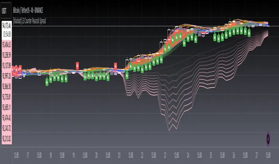
[blackcat] L3 Counter Peacock Spread█ OVERVIEW
The script titled " L3 Counter Peacock Spread" is an indicator designed for use in TradingView. It calculates and plots various moving averages, K lines derived from these moving averages, additional simple moving averages (SMAs), weighted moving averages (WMAs), and other technical indicators like slope calculations. The primary function of the script is to provide a comprehensive set of visual tools that traders can use to identify trends, potential support/resistance levels, and crossover signals.
█ LOGICAL FRAMEWORK
Input Parameters:
There are no explicit input parameters defined; all variables are hardcoded or calculated within the script.
Calculations:
• Moving Averages: Calculates Simple Moving Averages (SMA) using ta.sma.
• Slope Calculation: Computes the slope of a given series over a specified period using linear regression (ta.linreg).
• K Lines: Defines multiple exponentially adjusted SMAs based on a 30-period MA and a 1-period MA.
• Weighted Moving Average (WMA): Custom function to compute WMAs by iterating through price data points.
• Other Indicators: Includes Exponential Moving Average (EMA) for momentum calculation.
Plotting:
Various elements such as MAs, K lines, conditional bands, additional SMAs, and WMAs are plotted on the chart overlaying the main price action.
No loops control the behavior beyond those used in custom functions for calculating WMAs. Conditional statements determine the coloring of certain plot lines based on specific criteria.
█ CUSTOM FUNCTIONS
calculate_slope(src, length) :
• Purpose: To calculate the slope of a time-series data point over a specified number of periods.
• Functionality: Uses linear regression to find the current and previous slopes and computes their difference scaled by the timeframe multiplier.
• Parameters:
– src: Source of the input data (e.g., closing prices).
– length: Periodicity of the linreg calculation.
• Return Value: Computed slope value.
calculate_ma(source, length) :
• Purpose: To calculate the Simple Moving Average (SMA) of a given source over a specified period.
• Functionality: Utilizes TradingView’s built-in ta.sma function.
• Parameters:
– source: Input data series (e.g., closing prices).
– length: Number of bars considered for the SMA calculation.
• Return Value: Calculated SMA value.
calculate_k_lines(ma30, ma1) :
• Purpose: Generates multiple exponentially adjusted versions of a 30-period MA relative to a 1-period MA.
• Functionality: Multiplies the 30-period MA by coefficients ranging from 1.1 to 3 and subtracts multiples of the 1-period MA accordingly.
• Parameters:
– ma30: 30-period Simple Moving Average.
– ma1: 1-period Simple Moving Average.
• Return Value: Returns an array containing ten different \u2003\u2022 "K line" values.
calculate_wma(source, length) :
• Purpose: Computes the Weighted Moving Average (WMA) of a provided series over a defined period.
• Functionality: Iterates backward through the last 'n' bars, weights each bar according to its position, sums them up, and divides by the total weight.
• Parameters:
– source: Price series to average.
– length: Length of the lookback window.
• Return Value: Calculated WMA value.
█ KEY POINTS AND TECHNIQUES
• Advanced Pine Script Features: Utilization of custom functions for encapsulating complex logic, leveraging TradingView’s library functions (ta.sma, ta.linreg, ta.ema) for efficient computations.
• Optimization Techniques: Efficient computation of K lines via pre-calculated components (multiples of MA30 and MA1). Use of arrays to store intermediate results which simplifies plotting.
• Best Practices: Clear separation between calculation and visualization sections enhances readability and maintainability. Usage of color.new() allows dynamic adjustments without hardcoding colors directly into plot commands.
• Unique Approaches: Introduction of K lines provides an alternative representation of trend strength compared to traditional MAs. Implementation of conditional band coloring adds real-time context to existing visual cues.
█ EXTENDED KNOWLEDGE AND APPLICATIONS
Potential Modifications/Extensions:
• Adding more user-defined inputs for lengths of MAs, K lines, etc., would make the script more flexible.
• Incorporating alert conditions based on crossovers between key lines could enhance automated trading strategies.
Application Scenarios:
• Useful for both intraday and swing trading due to the combination of short-term and long-term MAs along with trend analysis via slopes and K lines.
• Can be integrated into larger systems combining this indicator with others like oscillators or volume-based metrics.
Related Concepts:
• Understanding how linear regression works internally aids in grasping the slope calculation.
• Familiarity with WMA versus SMA helps appreciate why different types of averaging might be necessary depending on market dynamics.
• Knowledge of candlestick patterns can complement insights gained from this indicator.
Pressure Zones with MA [SYNC & TRADE]Description:
The "Pressure Zones with MA " indicator is designed to analyze the pressure of buyers and sellers on the market, as well as to identify areas of increased activity. When designing it, the main task was to see manipulations on the market, when the power of sellers or the power of buyers is in a sideways trend or falling, and the opposite is growing.
Here is a good example. The power of sellers is in a narrow sideways trend, and sales are increasing very aggressively. The power of buyers is in a gray block with the inscription "range". Then we see the fading of the power of sellers and buyers furiously pounce on the asset that has fallen in price.
Here are the main aspects of its operation and use:
First, turn off the moving averages in the indicator settings, on the "style" tab. Choose your favorite asset, which you understand well and know all its ups and downs. I want you to see a clean chart, so that you can be imbued with a new idea, you need to watch it. This is a proprietary indicator and I understand that it does not have the inscription “buy” / “sell”, but believe me, if you pay attention, you will see its strength. I usually add functionality later, but the light code and visualization remain preferable in the first version.
Purpose:
The indicator helps to determine the strength of buyers and sellers in the market.
It visualizes zones where the pressure of buyers or sellers prevails.
Additionally displays moving averages (MA) for data smoothing.
Main components:
Buyer strength chart (blue line)
Seller strength chart (red line)
Moving averages for buyer and seller strength
Threshold line for defining zones
Indicator settings:
Period: defines the base period for calculations (default 89)
Threshold: sets the level for defining pressure zones (from 0 to 2, default 0.8)
MA type for purchases and sales: select the type of moving average (SMA, EMA, RMA, WMA, VWMA, HMA)
MA length for purchases and sales: period for calculating moving averages
Colors for uptrends and downtrends of MA
Moving averages:
Help smooth out data and identify trends
The direction of the MA (up or down) further confirms the current trend
The color of the MA changes depending on the direction (blue for up, red for down)
Now you can turn them on and see how they help in understanding where one or another force is weakening. It is in this case that we see the intersection of forces and the sellers' force is moving aggressively upward. Also, according to the moving average, we see the weakening of the sellers' force. The buyers' force was in the sideways range and then switched on to buy out and also according to the moving average, it is clear where the main interest in purchases disappeared.
Use:
Observe the strength of buyers and sellers relative to each other. They can move simultaneously in one direction, this is regarded as balance
can move in different directions and this will strengthen the upward force of sellers or buyers
You may also notice that the movement of one of the forces will be in a narrow range and the second will grow strongly - this is manipulation or trading without resistance.
You can also play with the threshold line, but it is not the main thing here. I disabled this function in the code.
// Display zones
//bgcolor(buy_zone ? color.new(color.blue, 90) : na)
//bgcolor(sell_zone ? color.new(color.red, 90) : na)
If you want to enable it, copy it instead
// Display zones
bgcolor(buy_zone ? color.new(color.blue, 90) : na)
bgcolor(sell_zone ? color.new(color.red, 90) : na)
Pay attention to the intersection of forces.
Use crossovers of force lines and their moving averages as potential signals
Combine the indicator signals with other technical analysis tools for confirmation
Limitations:
Requires customization of parameters for a specific trading instrument and timeframe
The indicator should not be used as the only tool for making trading decisions
Remember that this indicator provides additional information for market analysis, but is not a guarantee of successful trades. Always combine it with other analysis methods and follow risk management rules.
Описание:
Индикатор "Pressure Zones with MA " предназначен для анализа давления покупателей и продавцов на рынке, а также для определения зон повышенной активности. При его проектировании основная задача была увидеть манипуляции на рынке, когда сила продавцов или сила покупателей стоит в боковике или падает, а противоположная растет.
Вот хороший пример. Сила продавцов стоит в узком боковике, а продажи очень агрессивно усиливаются. Сила покупателей в сером блоке с надписью “range”. Потом мы видим затухание силы продавцов и покупателей яростно накидываются на подешевевший актив.
Вот основные аспекты его работы и использования:
Для начала отключите средние скользящие в настройках индикатора, на закладке “стиль”. Выберите свой любимый актив, в котором вы хорошо разбираетесь и знаете его все взлеты и падения. Я хочу чтобы вы увидели чистый график, для того чтобы вы могли проникнутся новой идеей нужно понаблюдать за ним. Это авторский индикатор и я понимаю что на нем нет надписи “купить” / “продать”, но поверьте уделив свое внимание вы увидите его силу. Я обычно потом добавляю функционал но легкий код и визуализация, в первом варианте остается предпочтительней.
Назначение:
Индикатор помогает определить силу покупателей и продавцов на рынке.
Он визуализирует зоны, где преобладает давление покупателей или продавцов.
Дополнительно отображает скользящие средние (MA) для сглаживания данных.
Основные компоненты:
График силы покупателей (синяя линия)
График силы продавцов (красная линия)
Скользящие средние для силы покупателей и продавцов
Пороговая линия для определения зон
Настройки индикатора:
Период (Period): определяет базовый период для расчетов (по умолчанию 89)
Порог (Threshold): устанавливает уровень для определения зон давления (от 0 до 2, по умолчанию 0.8)
Тип MA для покупок и продаж: выбор типа скользящей средней (SMA, EMA, RMA, WMA, VWMA, HMA)
Длина MA для покупок и продаж: период для расчета скользящих средних
Цвета для восходящего и нисходящего трендов MA
Скользящие средние:
Помогают сглаживать данные и выявлять тренды
Направление MA (вверх или вниз) дополнительно подтверждает текущий тренд
Цвет MA меняется в зависимости от направления (синий для восходящего, красный для нисходящего)
Теперь вы можете их включить и посмотреть как они помогают в понимании где ослабевает та или иная сила. Именно в этом случае мы видим пересечение сил и сила продавцов идет агрессивно вверх. Также по средней скользящей мы видим затухание силы продавцов. Сила покупателей стояла в боковике потом включилась на откуп и также по средней скользящей видно где пропал основной интерес к покупкам.
Использование:
Наблюдайте за силой покупателей и продавцов относительно друг друга. Они могут двигаться одновременно в одном направлении это расценивается как баланс
могут двигаться в разных направлениях и это будет усиливать восходящую силу продавцов или покупателей
также возможно вы заметите что движение одной из силы будет в узком диапазоне а вторая будет сильно расти - это манипуляция или торговля без сопротивления.
Также можете поиграть с пороговой линией, но она совершенно не главная здесь. В коде я отключил эту функцию.
// Display zones
//bgcolor(buy_zone ? color.new(color.blue, 90) : na)
//bgcolor(sell_zone ? color.new(color.red, 90) : na)
Если захотите включить скопируйте вместо нее
// Display zones
bgcolor(buy_zone ? color.new(color.blue, 90) : na)
bgcolor(sell_zone ? color.new(color.red, 90) : na)
Обращайте внимание на пересечение сил.
Используйте пересечения линий силы и их скользящих средних как потенциальные сигналы
Комбинируйте сигналы индикатора с другими инструментами технического анализа для подтверждения
Ограничения:
Требуется настройка параметров под конкретный торговый инструмент и таймфрейм
Не следует использовать индикатор как единственный инструмент для принятия торговых решений
Помните, что этот индикатор предоставляет дополнительную информацию для анализа рынка, но не является гарантией успешных сделок. Всегда сочетайте его с другими методами анализа и соблюдайте правила управления рисками.

Combined IndicatorSummary
This custom Pine Script combines three main indicators into one, each with its own functionalities and visual cues. It provides a comprehensive approach to trend analysis by integrating short-term, medium-term, and long-term indicators. Each part of the indicator can be toggled on or off independently to suit the trader’s needs.
Part 1: EMA 14 and EMA 200
Purpose: This part of the indicator is designed to identify short-term and long-term trends using Exponential Moving Averages (EMA). It helps traders spot potential entry and exit points based on the relationship between short-term and long-term moving averages.
Visuals:
• EMA 14: Plotted in blue (#2962ff)
• EMA 200: Plotted in red (#f23645)
Signals:
• Long Signal: Generated when EMA 14 crosses above EMA 200, indicating a potential upward trend.
• Short Signal: Generated when EMA 14 crosses below EMA 200, indicating a potential downward trend.
Usage: Toggle this part on or off using the checkbox input to focus on short-term vs. long-term trends.
Part 2: EMA 9 and SMA 20
Purpose: This part combines Exponential and Simple Moving Averages to provide a medium-term trend analysis. It helps smooth out price data and identify potential trend reversals and continuation patterns.
Visuals:
• EMA 9: Plotted in green
• SMA 20: Plotted in dark red
Usage: Toggle this part on or off using the checkbox input to focus on medium-term trends and price smoothing.
Part 3: Golden Cross and Death Cross
Purpose: This part identifies long-term bullish and bearish market conditions using the 50-day and 200-day Simple Moving Averages (SMA). It highlights major trend changes that can inform long-term investment decisions.
Visuals:
• 50-day SMA: Plotted in gold (#ffe600)
• 200-day SMA: Plotted in black
Signals:
• Golden Cross: Generated when the 50-day SMA crosses above the 200-day SMA, indicating a potential long-term upward trend.
• Death Cross: Generated when the 50-day SMA crosses below the 200-day SMA, indicating a potential long-term downward trend.
Usage: Toggle this part on or off using the checkbox input to focus on long-term trend changes.
How to Use
1. Enable/Disable Indicators: Use the checkboxes provided in the input settings to enable or disable each part of the indicator according to your analysis needs.
2. Interpret Signals: Look for crossover events to determine potential entry and exit points based on the relationship between the moving averages.
3. Visual Confirmation: Use the color-coded lines and shape markers on the chart to visually confirm signals and trends.
4. Customize Settings: Adjust the lengths of the EMAs and SMAs in the input settings to suit your trading strategy and the specific asset you are analyzing.
Practical Application
• Short-Term Trading: Use the EMA 14 and EMA 200 signals to identify quick trend changes.
• Medium-Term Trading: Use the EMA 9 and SMA 20 to capture medium-term trends and reversals.
• Long-Term Investing: Monitor the Golden Cross and Death Cross signals to make decisions based on long-term trend changes.
Example of Unique Features
• Integrated Toggle System: Allows users to enable or disable specific parts of the indicator to customize their analysis.
• Multi-Tier Trend Analysis: Combines short-term, medium-term, and long-term indicators to provide a comprehensive view of the market.
Triple Moving Average CrossoverBelow is the Pine Script code for TradingView that creates an indicator with three user-defined moving averages (with default periods of 10, 50, and 100) and labels for buy and sell signals at key crossovers. Additionally, it creates a label if the price increases by 100 points from the buy entry or decreases by 100 points from the sell entry, with the label saying "+100".
Explanation:
Indicator Definition: indicator("Triple Moving Average Crossover", overlay=true) defines the script as an indicator that overlays on the chart.
User Inputs: input.int functions allow users to define the periods for the short, middle, and long moving averages with defaults of 10, 50, and 100, respectively.
Moving Averages Calculation: The ta.sma function calculates the simple moving averages for the specified periods.
Plotting Moving Averages: plot functions plot the short, middle, and long moving averages on the chart with blue, orange, and red colors.
Crossover Detection: ta.crossover and ta.crossunder functions detect when the short moving average crosses above or below the middle moving average and when the middle moving average crosses above or below the long moving average.
Entry Price Tracking: Variables buyEntryPrice and sellEntryPrice store the buy and sell entry prices. These prices are updated whenever a bullish or bearish crossover occurs.
100 Points Move Detection: buyTargetReached checks if the current price has increased by 100 points from the buy entry price. sellTargetReached checks if the current price has decreased by 100 points from the sell entry price.
Plotting Labels: plotshape functions plot the buy and sell labels at the crossovers and the +100 labels when the target moves are reached. The labels are displayed in white and green colors.
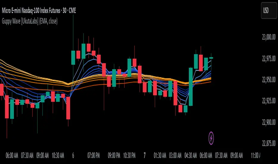
Guppy Wave [UkutaLabs]█ OVERVIEW
The Guppy Wave Indicator is a collection of Moving Averages that provide insight on current market strength. This is done by plotting a series of 12 Moving Averages and analysing where each one is positioned relative to the others.
In doing this, this script is able to identify short-term moves and give an idea of the current strength and direction of the market.
The aim of this script is to simplify the trading experience of users by automatically displaying a series of useful Moving Averages to provide insight into short-term market strength.
█ USAGE
The Guppy Wave is generated using a series of 12 total Moving Averages composed of 6 Small-Period Moving Averages and 6 Large Period Moving Averages. By measuring the position of each moving average relative to the others, this script provides unique insight into the current strength of the market.
Rather than simply plotting 12 Moving Averages, a color gradient is instead drawn between the Moving Averages to make it easier to visualise the distribution of the Guppy Wave. The color of this gradient changes depending on whether the Small-Period Averages are above or below the Large-Period Averages, allowing traders to see current short-term market strength at a glance.
When the gradient fans out, this indicates a rapid short-term move. When the gradient is thin, this indicates that there is no dominant power in the market.
█ SETTINGS
• Moving Average Type: Determines the type of Moving Average that get plotted (EMA, SMA, WMA, VWMA, HMA, RMA)
• Moving Average Source: Determines the source price used to calculate Moving Averages (open, high, low, close, hl2, hlc3, ohlc4, hlcc4)
• Bearish Color: Determines the color of the gradient when Small-Period MAs are above Large-Period MAs.
• Bullish Color: Determines the color of the gradient when Small-Period MAs are below Large-Period MAs.
Johnny's Adjusted BB Buy/Sell Signal"Johnny's Adjusted BB Buy/Sell Signal" leverages Bollinger Bands and moving averages to provide dynamic buy and sell signals based on market conditions. This indicator is particularly useful for traders looking to identify strategic entry and exit points based on volatility and trend analysis.
How It Works
Bollinger Bands Setup: The indicator calculates Bollinger Bands using a specified length and multiplier. These bands serve to identify potential overbought (upper band) or oversold (lower band) conditions.
Moving Averages: Two moving averages are calculated — a trend moving average (trendMA) and a long-term moving average (longTermMA) — to gauge the market's direction over different time frames.
Market Phase Determination: The script classifies the market into bullish or bearish phases based on the relationship of the closing price to the long-term moving average.
Strong Buy and Sell Signals: Enhanced signals are generated based on how significantly the price deviates from the Bollinger Bands, coupled with the average candle size over a specified lookback period. The signals are adjusted based on whether the market is bullish or bearish:
In bullish markets, a strong buy signal is triggered if the price significantly drops below the lower Bollinger Band. Conversely, a strong sell signal is activated when the price rises well above the upper band.
In bearish markets, these signals are modified to be more conservative, adjusting the thresholds for triggering strong buy and sell signals.
Features:
Flexibility: Users can adjust the length of the Bollinger Bands and moving averages, as well as the multipliers and factors that determine the strength of buy and sell signals, making it highly customizable to different trading styles and market conditions.
Visual Aids: The script vividly plots the Bollinger Bands and moving averages, and signals are visually represented on the chart, allowing traders to quickly assess trading opportunities:
Regular buy and sell signals are indicated by simple shapes below or above price bars.
Strong buy and sell signals are highlighted with distinctive colors and placed prominently to catch the trader's attention.
Background Coloring: The background color changes based on the market phase, providing an immediate visual cue of the market's overall sentiment.
Usage:
This indicator is ideal for traders who rely on technical analysis to guide their trading decisions. By integrating both Bollinger Bands and moving averages, it provides a multi-faceted view of market trends and volatility, making it suitable for identifying potential reversals and continuation patterns. Traders can use this tool to enhance their understanding of market dynamics and refine their trading strategies accordingly.

[KVA] Extremes ProfilerExtremes Profiler is a specialized indicator crafted for traders focusing on the relationship between price extremes and moving averages. This tool offers a comprehensive perspective on price dynamics by quantifying and visualizing significant distances of current prices from various moving averages. It effectively highlights the top extremes in market movements, providing key insights into price extremities relative to these averages. The indicator's ability to analyze and display these distances makes it a valuable tool for understanding market trends and potential turning points. Traders can leverage the Extremes Profiler to gain a deeper understanding of how prices behave in relation to commonly watched moving averages, thus aiding in making informed trading decisions
Key Features :
Extensive MA Analysis : Tracks the price distance from multiple moving averages including EMA, SMA, WMA, RMA, and HMA.
Top 50 (100) Distance Metrics : Highlights the 50 (100)greatest (highest or lowest) distances from each selected MA, pinpointing significant market deviations.
Customizable Periods : Offers flexibility with adjustable periods to align with diverse trading strategies.
Comprehensive View : Switch between timeframes for a well-rounded understanding of short-term fluctuations and long-term market trends.
Cross-Asset Comparison : Utilize the indicator to compare different assets, gaining insights into the relative dynamics and volatility of various markets. By analyzing multiple assets, traders can discern broader market trends and better understand asset-specific behaviors.
Customizable Display : Users can adjust the periods and number of results to suit their analytical needs.

STD-Adaptive T3 [Loxx]STD-Adaptive T3 is a standard deviation adaptive T3 moving average filter. This indicator acts more like a trend overlay indicator with gradient coloring.
What is the T3 moving average?
Better Moving Averages Tim Tillson
November 1, 1998
Tim Tillson is a software project manager at Hewlett-Packard, with degrees in Mathematics and Computer Science. He has privately traded options and equities for 15 years.
Introduction
"Digital filtering includes the process of smoothing, predicting, differentiating, integrating, separation of signals, and removal of noise from a signal. Thus many people who do such things are actually using digital filters without realizing that they are; being unacquainted with the theory, they neither understand what they have done nor the possibilities of what they might have done."
This quote from R. W. Hamming applies to the vast majority of indicators in technical analysis . Moving averages, be they simple, weighted, or exponential, are lowpass filters; low frequency components in the signal pass through with little attenuation, while high frequencies are severely reduced.
"Oscillator" type indicators (such as MACD , Momentum, Relative Strength Index ) are another type of digital filter called a differentiator.
Tushar Chande has observed that many popular oscillators are highly correlated, which is sensible because they are trying to measure the rate of change of the underlying time series, i.e., are trying to be the first and second derivatives we all learned about in Calculus.
We use moving averages (lowpass filters) in technical analysis to remove the random noise from a time series, to discern the underlying trend or to determine prices at which we will take action. A perfect moving average would have two attributes:
It would be smooth, not sensitive to random noise in the underlying time series. Another way of saying this is that its derivative would not spuriously alternate between positive and negative values.
It would not lag behind the time series it is computed from. Lag, of course, produces late buy or sell signals that kill profits.
The only way one can compute a perfect moving average is to have knowledge of the future, and if we had that, we would buy one lottery ticket a week rather than trade!
Having said this, we can still improve on the conventional simple, weighted, or exponential moving averages. Here's how:
Two Interesting Moving Averages
We will examine two benchmark moving averages based on Linear Regression analysis.
In both cases, a Linear Regression line of length n is fitted to price data.
I call the first moving average ILRS, which stands for Integral of Linear Regression Slope. One simply integrates the slope of a linear regression line as it is successively fitted in a moving window of length n across the data, with the constant of integration being a simple moving average of the first n points. Put another way, the derivative of ILRS is the linear regression slope. Note that ILRS is not the same as a SMA ( simple moving average ) of length n, which is actually the midpoint of the linear regression line as it moves across the data.
We can measure the lag of moving averages with respect to a linear trend by computing how they behave when the input is a line with unit slope. Both SMA (n) and ILRS(n) have lag of n/2, but ILRS is much smoother than SMA .
Our second benchmark moving average is well known, called EPMA or End Point Moving Average. It is the endpoint of the linear regression line of length n as it is fitted across the data. EPMA hugs the data more closely than a simple or exponential moving average of the same length. The price we pay for this is that it is much noisier (less smooth) than ILRS, and it also has the annoying property that it overshoots the data when linear trends are present.
However, EPMA has a lag of 0 with respect to linear input! This makes sense because a linear regression line will fit linear input perfectly, and the endpoint of the LR line will be on the input line.
These two moving averages frame the tradeoffs that we are facing. On one extreme we have ILRS, which is very smooth and has considerable phase lag. EPMA has 0 phase lag, but is too noisy and overshoots. We would like to construct a better moving average which is as smooth as ILRS, but runs closer to where EPMA lies, without the overshoot.
A easy way to attempt this is to split the difference, i.e. use (ILRS(n)+EPMA(n))/2. This will give us a moving average (call it IE /2) which runs in between the two, has phase lag of n/4 but still inherits considerable noise from EPMA. IE /2 is inspirational, however. Can we build something that is comparable, but smoother? Figure 1 shows ILRS, EPMA, and IE /2.
Filter Techniques
Any thoughtful student of filter theory (or resolute experimenter) will have noticed that you can improve the smoothness of a filter by running it through itself multiple times, at the cost of increasing phase lag.
There is a complementary technique (called twicing by J.W. Tukey) which can be used to improve phase lag. If L stands for the operation of running data through a low pass filter, then twicing can be described by:
L' = L(time series) + L(time series - L(time series))
That is, we add a moving average of the difference between the input and the moving average to the moving average. This is algebraically equivalent to:
2L-L(L)
This is the Double Exponential Moving Average or DEMA , popularized by Patrick Mulloy in TASAC (January/February 1994).
In our taxonomy, DEMA has some phase lag (although it exponentially approaches 0) and is somewhat noisy, comparable to IE /2 indicator.
We will use these two techniques to construct our better moving average, after we explore the first one a little more closely.
Fixing Overshoot
An n-day EMA has smoothing constant alpha=2/(n+1) and a lag of (n-1)/2.
Thus EMA (3) has lag 1, and EMA (11) has lag 5. Figure 2 shows that, if I am willing to incur 5 days of lag, I get a smoother moving average if I run EMA (3) through itself 5 times than if I just take EMA (11) once.
This suggests that if EPMA and DEMA have 0 or low lag, why not run fast versions (eg DEMA (3)) through themselves many times to achieve a smooth result? The problem is that multiple runs though these filters increase their tendency to overshoot the data, giving an unusable result. This is because the amplitude response of DEMA and EPMA is greater than 1 at certain frequencies, giving a gain of much greater than 1 at these frequencies when run though themselves multiple times. Figure 3 shows DEMA (7) and EPMA(7) run through themselves 3 times. DEMA^3 has serious overshoot, and EPMA^3 is terrible.
The solution to the overshoot problem is to recall what we are doing with twicing:
DEMA (n) = EMA (n) + EMA (time series - EMA (n))
The second term is adding, in effect, a smooth version of the derivative to the EMA to achieve DEMA . The derivative term determines how hot the moving average's response to linear trends will be. We need to simply turn down the volume to achieve our basic building block:
EMA (n) + EMA (time series - EMA (n))*.7;
This is algebraically the same as:
EMA (n)*1.7-EMA( EMA (n))*.7;
I have chosen .7 as my volume factor, but the general formula (which I call "Generalized Dema") is:
GD (n,v) = EMA (n)*(1+v)-EMA( EMA (n))*v,
Where v ranges between 0 and 1. When v=0, GD is just an EMA , and when v=1, GD is DEMA . In between, GD is a cooler DEMA . By using a value for v less than 1 (I like .7), we cure the multiple DEMA overshoot problem, at the cost of accepting some additional phase delay. Now we can run GD through itself multiple times to define a new, smoother moving average T3 that does not overshoot the data:
T3(n) = GD ( GD ( GD (n)))
In filter theory parlance, T3 is a six-pole non-linear Kalman filter. Kalman filters are ones which use the error (in this case (time series - EMA (n)) to correct themselves. In Technical Analysis , these are called Adaptive Moving Averages; they track the time series more aggressively when it is making large moves.
Included
Bar coloring
Loxx's Expanded Source Types

Softmax Normalized T3 Histogram [Loxx]Softmax Normalized T3 Histogram is a T3 moving average that is morphed into a normalized oscillator from -1 to 1.
What is the Softmax function?
The softmax function, also known as softargmax: or normalized exponential function, converts a vector of K real numbers into a probability distribution of K possible outcomes. It is a generalization of the logistic function to multiple dimensions, and used in multinomial logistic regression. The softmax function is often used as the last activation function of a neural network to normalize the output of a network to a probability distribution over predicted output classes, based on Luce's choice axiom.
What is the T3 moving average?
Better Moving Averages Tim Tillson
November 1, 1998
Tim Tillson is a software project manager at Hewlett-Packard, with degrees in Mathematics and Computer Science. He has privately traded options and equities for 15 years.
Introduction
"Digital filtering includes the process of smoothing, predicting, differentiating, integrating, separation of signals, and removal of noise from a signal. Thus many people who do such things are actually using digital filters without realizing that they are; being unacquainted with the theory, they neither understand what they have done nor the possibilities of what they might have done."
This quote from R. W. Hamming applies to the vast majority of indicators in technical analysis . Moving averages, be they simple, weighted, or exponential, are lowpass filters; low frequency components in the signal pass through with little attenuation, while high frequencies are severely reduced.
"Oscillator" type indicators (such as MACD , Momentum, Relative Strength Index ) are another type of digital filter called a differentiator.
Tushar Chande has observed that many popular oscillators are highly correlated, which is sensible because they are trying to measure the rate of change of the underlying time series, i.e., are trying to be the first and second derivatives we all learned about in Calculus.
We use moving averages (lowpass filters) in technical analysis to remove the random noise from a time series, to discern the underlying trend or to determine prices at which we will take action. A perfect moving average would have two attributes:
It would be smooth, not sensitive to random noise in the underlying time series. Another way of saying this is that its derivative would not spuriously alternate between positive and negative values.
It would not lag behind the time series it is computed from. Lag, of course, produces late buy or sell signals that kill profits.
The only way one can compute a perfect moving average is to have knowledge of the future, and if we had that, we would buy one lottery ticket a week rather than trade!
Having said this, we can still improve on the conventional simple, weighted, or exponential moving averages. Here's how:
Two Interesting Moving Averages
We will examine two benchmark moving averages based on Linear Regression analysis.
In both cases, a Linear Regression line of length n is fitted to price data.
I call the first moving average ILRS, which stands for Integral of Linear Regression Slope. One simply integrates the slope of a linear regression line as it is successively fitted in a moving window of length n across the data, with the constant of integration being a simple moving average of the first n points. Put another way, the derivative of ILRS is the linear regression slope. Note that ILRS is not the same as a SMA ( simple moving average ) of length n, which is actually the midpoint of the linear regression line as it moves across the data.
We can measure the lag of moving averages with respect to a linear trend by computing how they behave when the input is a line with unit slope. Both SMA (n) and ILRS(n) have lag of n/2, but ILRS is much smoother than SMA .
Our second benchmark moving average is well known, called EPMA or End Point Moving Average. It is the endpoint of the linear regression line of length n as it is fitted across the data. EPMA hugs the data more closely than a simple or exponential moving average of the same length. The price we pay for this is that it is much noisier (less smooth) than ILRS, and it also has the annoying property that it overshoots the data when linear trends are present.
However, EPMA has a lag of 0 with respect to linear input! This makes sense because a linear regression line will fit linear input perfectly, and the endpoint of the LR line will be on the input line.
These two moving averages frame the tradeoffs that we are facing. On one extreme we have ILRS, which is very smooth and has considerable phase lag. EPMA has 0 phase lag, but is too noisy and overshoots. We would like to construct a better moving average which is as smooth as ILRS, but runs closer to where EPMA lies, without the overshoot.
A easy way to attempt this is to split the difference, i.e. use (ILRS(n)+EPMA(n))/2. This will give us a moving average (call it IE /2) which runs in between the two, has phase lag of n/4 but still inherits considerable noise from EPMA. IE /2 is inspirational, however. Can we build something that is comparable, but smoother? Figure 1 shows ILRS, EPMA, and IE /2.
Filter Techniques
Any thoughtful student of filter theory (or resolute experimenter) will have noticed that you can improve the smoothness of a filter by running it through itself multiple times, at the cost of increasing phase lag.
There is a complementary technique (called twicing by J.W. Tukey) which can be used to improve phase lag. If L stands for the operation of running data through a low pass filter, then twicing can be described by:
L' = L(time series) + L(time series - L(time series))
That is, we add a moving average of the difference between the input and the moving average to the moving average. This is algebraically equivalent to:
2L-L(L)
This is the Double Exponential Moving Average or DEMA , popularized by Patrick Mulloy in TASAC (January/February 1994).
In our taxonomy, DEMA has some phase lag (although it exponentially approaches 0) and is somewhat noisy, comparable to IE /2 indicator.
We will use these two techniques to construct our better moving average, after we explore the first one a little more closely.
Fixing Overshoot
An n-day EMA has smoothing constant alpha=2/(n+1) and a lag of (n-1)/2.
Thus EMA (3) has lag 1, and EMA (11) has lag 5. Figure 2 shows that, if I am willing to incur 5 days of lag, I get a smoother moving average if I run EMA (3) through itself 5 times than if I just take EMA (11) once.
This suggests that if EPMA and DEMA have 0 or low lag, why not run fast versions (eg DEMA (3)) through themselves many times to achieve a smooth result? The problem is that multiple runs though these filters increase their tendency to overshoot the data, giving an unusable result. This is because the amplitude response of DEMA and EPMA is greater than 1 at certain frequencies, giving a gain of much greater than 1 at these frequencies when run though themselves multiple times. Figure 3 shows DEMA (7) and EPMA(7) run through themselves 3 times. DEMA^3 has serious overshoot, and EPMA^3 is terrible.
The solution to the overshoot problem is to recall what we are doing with twicing:
DEMA (n) = EMA (n) + EMA (time series - EMA (n))
The second term is adding, in effect, a smooth version of the derivative to the EMA to achieve DEMA . The derivative term determines how hot the moving average's response to linear trends will be. We need to simply turn down the volume to achieve our basic building block:
EMA (n) + EMA (time series - EMA (n))*.7;
This is algebraically the same as:
EMA (n)*1.7-EMA( EMA (n))*.7;
I have chosen .7 as my volume factor, but the general formula (which I call "Generalized Dema") is:
GD (n,v) = EMA (n)*(1+v)-EMA( EMA (n))*v,
Where v ranges between 0 and 1. When v=0, GD is just an EMA , and when v=1, GD is DEMA . In between, GD is a cooler DEMA . By using a value for v less than 1 (I like .7), we cure the multiple DEMA overshoot problem, at the cost of accepting some additional phase delay. Now we can run GD through itself multiple times to define a new, smoother moving average T3 that does not overshoot the data:
T3(n) = GD ( GD ( GD (n)))
In filter theory parlance, T3 is a six-pole non-linear Kalman filter. Kalman filters are ones which use the error (in this case (time series - EMA (n)) to correct themselves. In Technical Analysis , these are called Adaptive Moving Averages; they track the time series more aggressively when it is making large moves.
Included:
Bar coloring
Signals
Alerts
Loxx's Expanded Source Types
T3 Velocity Candles [Loxx]T3 Velocity Candles is a candle coloring overlay that calculates its gradient coloring using T3 velocity.
What is the T3 moving average?
Better Moving Averages Tim Tillson
November 1, 1998
Tim Tillson is a software project manager at Hewlett-Packard, with degrees in Mathematics and Computer Science. He has privately traded options and equities for 15 years.
Introduction
"Digital filtering includes the process of smoothing, predicting, differentiating, integrating, separation of signals, and removal of noise from a signal. Thus many people who do such things are actually using digital filters without realizing that they are; being unacquainted with the theory, they neither understand what they have done nor the possibilities of what they might have done."
This quote from R. W. Hamming applies to the vast majority of indicators in technical analysis . Moving averages, be they simple, weighted, or exponential, are lowpass filters; low frequency components in the signal pass through with little attenuation, while high frequencies are severely reduced.
"Oscillator" type indicators (such as MACD , Momentum, Relative Strength Index ) are another type of digital filter called a differentiator.
Tushar Chande has observed that many popular oscillators are highly correlated, which is sensible because they are trying to measure the rate of change of the underlying time series, i.e., are trying to be the first and second derivatives we all learned about in Calculus.
We use moving averages (lowpass filters) in technical analysis to remove the random noise from a time series, to discern the underlying trend or to determine prices at which we will take action. A perfect moving average would have two attributes:
It would be smooth, not sensitive to random noise in the underlying time series. Another way of saying this is that its derivative would not spuriously alternate between positive and negative values.
It would not lag behind the time series it is computed from. Lag, of course, produces late buy or sell signals that kill profits.
The only way one can compute a perfect moving average is to have knowledge of the future, and if we had that, we would buy one lottery ticket a week rather than trade!
Having said this, we can still improve on the conventional simple, weighted, or exponential moving averages. Here's how:
Two Interesting Moving Averages
We will examine two benchmark moving averages based on Linear Regression analysis.
In both cases, a Linear Regression line of length n is fitted to price data.
I call the first moving average ILRS, which stands for Integral of Linear Regression Slope. One simply integrates the slope of a linear regression line as it is successively fitted in a moving window of length n across the data, with the constant of integration being a simple moving average of the first n points. Put another way, the derivative of ILRS is the linear regression slope. Note that ILRS is not the same as a SMA ( simple moving average ) of length n, which is actually the midpoint of the linear regression line as it moves across the data.
We can measure the lag of moving averages with respect to a linear trend by computing how they behave when the input is a line with unit slope. Both SMA (n) and ILRS(n) have lag of n/2, but ILRS is much smoother than SMA .
Our second benchmark moving average is well known, called EPMA or End Point Moving Average. It is the endpoint of the linear regression line of length n as it is fitted across the data. EPMA hugs the data more closely than a simple or exponential moving average of the same length. The price we pay for this is that it is much noisier (less smooth) than ILRS, and it also has the annoying property that it overshoots the data when linear trends are present.
However, EPMA has a lag of 0 with respect to linear input! This makes sense because a linear regression line will fit linear input perfectly, and the endpoint of the LR line will be on the input line.
These two moving averages frame the tradeoffs that we are facing. On one extreme we have ILRS, which is very smooth and has considerable phase lag. EPMA has 0 phase lag, but is too noisy and overshoots. We would like to construct a better moving average which is as smooth as ILRS, but runs closer to where EPMA lies, without the overshoot.
A easy way to attempt this is to split the difference, i.e. use (ILRS(n)+EPMA(n))/2. This will give us a moving average (call it IE /2) which runs in between the two, has phase lag of n/4 but still inherits considerable noise from EPMA. IE /2 is inspirational, however. Can we build something that is comparable, but smoother? Figure 1 shows ILRS, EPMA, and IE /2.
Filter Techniques
Any thoughtful student of filter theory (or resolute experimenter) will have noticed that you can improve the smoothness of a filter by running it through itself multiple times, at the cost of increasing phase lag.
There is a complementary technique (called twicing by J.W. Tukey) which can be used to improve phase lag. If L stands for the operation of running data through a low pass filter, then twicing can be described by:
L' = L(time series) + L(time series - L(time series))
That is, we add a moving average of the difference between the input and the moving average to the moving average. This is algebraically equivalent to:
2L-L(L)
This is the Double Exponential Moving Average or DEMA , popularized by Patrick Mulloy in TASAC (January/February 1994).
In our taxonomy, DEMA has some phase lag (although it exponentially approaches 0) and is somewhat noisy, comparable to IE /2 indicator.
We will use these two techniques to construct our better moving average, after we explore the first one a little more closely.
Fixing Overshoot
An n-day EMA has smoothing constant alpha=2/(n+1) and a lag of (n-1)/2.
Thus EMA (3) has lag 1, and EMA (11) has lag 5. Figure 2 shows that, if I am willing to incur 5 days of lag, I get a smoother moving average if I run EMA (3) through itself 5 times than if I just take EMA (11) once.
This suggests that if EPMA and DEMA have 0 or low lag, why not run fast versions (eg DEMA (3)) through themselves many times to achieve a smooth result? The problem is that multiple runs though these filters increase their tendency to overshoot the data, giving an unusable result. This is because the amplitude response of DEMA and EPMA is greater than 1 at certain frequencies, giving a gain of much greater than 1 at these frequencies when run though themselves multiple times. Figure 3 shows DEMA (7) and EPMA(7) run through themselves 3 times. DEMA^3 has serious overshoot, and EPMA^3 is terrible.
The solution to the overshoot problem is to recall what we are doing with twicing:
DEMA (n) = EMA (n) + EMA (time series - EMA (n))
The second term is adding, in effect, a smooth version of the derivative to the EMA to achieve DEMA . The derivative term determines how hot the moving average's response to linear trends will be. We need to simply turn down the volume to achieve our basic building block:
EMA (n) + EMA (time series - EMA (n))*.7;
This is algebraically the same as:
EMA (n)*1.7-EMA( EMA (n))*.7;
I have chosen .7 as my volume factor, but the general formula (which I call "Generalized Dema") is:
GD (n,v) = EMA (n)*(1+v)-EMA( EMA (n))*v,
Where v ranges between 0 and 1. When v=0, GD is just an EMA , and when v=1, GD is DEMA . In between, GD is a cooler DEMA . By using a value for v less than 1 (I like .7), we cure the multiple DEMA overshoot problem, at the cost of accepting some additional phase delay. Now we can run GD through itself multiple times to define a new, smoother moving average T3 that does not overshoot the data:
T3(n) = GD ( GD ( GD (n)))
In filter theory parlance, T3 is a six-pole non-linear Kalman filter. Kalman filters are ones which use the error (in this case (time series - EMA (n)) to correct themselves. In Technical Analysis , these are called Adaptive Moving Averages; they track the time series more aggressively when it is making large moves.

T3 Striped [Loxx]Theory:
Although T3 is widely used, some of the details on how it is calculated are less known. T3 has, internally, 6 "levels" or "steps" that it uses for its calculation.
This version:
Instead of showing the final T3 value, this indicator shows those intermediate steps. This shows the "building steps" of T3 and can be used for trend assessment as well as for possible support / resistance values.
What is the T3 moving average?
Better Moving Averages Tim Tillson
November 1, 1998
Tim Tillson is a software project manager at Hewlett-Packard, with degrees in Mathematics and Computer Science. He has privately traded options and equities for 15 years.
Introduction
"Digital filtering includes the process of smoothing, predicting, differentiating, integrating, separation of signals, and removal of noise from a signal. Thus many people who do such things are actually using digital filters without realizing that they are; being unacquainted with the theory, they neither understand what they have done nor the possibilities of what they might have done."
This quote from R. W. Hamming applies to the vast majority of indicators in technical analysis . Moving averages, be they simple, weighted, or exponential, are lowpass filters; low frequency components in the signal pass through with little attenuation, while high frequencies are severely reduced.
"Oscillator" type indicators (such as MACD , Momentum, Relative Strength Index ) are another type of digital filter called a differentiator.
Tushar Chande has observed that many popular oscillators are highly correlated, which is sensible because they are trying to measure the rate of change of the underlying time series, i.e., are trying to be the first and second derivatives we all learned about in Calculus.
We use moving averages (lowpass filters) in technical analysis to remove the random noise from a time series, to discern the underlying trend or to determine prices at which we will take action. A perfect moving average would have two attributes:
It would be smooth, not sensitive to random noise in the underlying time series. Another way of saying this is that its derivative would not spuriously alternate between positive and negative values.
It would not lag behind the time series it is computed from. Lag, of course, produces late buy or sell signals that kill profits.
The only way one can compute a perfect moving average is to have knowledge of the future, and if we had that, we would buy one lottery ticket a week rather than trade!
Having said this, we can still improve on the conventional simple, weighted, or exponential moving averages. Here's how:
Two Interesting Moving Averages
We will examine two benchmark moving averages based on Linear Regression analysis.
In both cases, a Linear Regression line of length n is fitted to price data.
I call the first moving average ILRS, which stands for Integral of Linear Regression Slope. One simply integrates the slope of a linear regression line as it is successively fitted in a moving window of length n across the data, with the constant of integration being a simple moving average of the first n points. Put another way, the derivative of ILRS is the linear regression slope. Note that ILRS is not the same as a SMA ( simple moving average ) of length n, which is actually the midpoint of the linear regression line as it moves across the data.
We can measure the lag of moving averages with respect to a linear trend by computing how they behave when the input is a line with unit slope. Both SMA (n) and ILRS(n) have lag of n/2, but ILRS is much smoother than SMA .
Our second benchmark moving average is well known, called EPMA or End Point Moving Average. It is the endpoint of the linear regression line of length n as it is fitted across the data. EPMA hugs the data more closely than a simple or exponential moving average of the same length. The price we pay for this is that it is much noisier (less smooth) than ILRS, and it also has the annoying property that it overshoots the data when linear trends are present.
However, EPMA has a lag of 0 with respect to linear input! This makes sense because a linear regression line will fit linear input perfectly, and the endpoint of the LR line will be on the input line.
These two moving averages frame the tradeoffs that we are facing. On one extreme we have ILRS, which is very smooth and has considerable phase lag. EPMA has 0 phase lag, but is too noisy and overshoots. We would like to construct a better moving average which is as smooth as ILRS, but runs closer to where EPMA lies, without the overshoot.
A easy way to attempt this is to split the difference, i.e. use (ILRS(n)+EPMA(n))/2. This will give us a moving average (call it IE /2) which runs in between the two, has phase lag of n/4 but still inherits considerable noise from EPMA. IE /2 is inspirational, however. Can we build something that is comparable, but smoother? Figure 1 shows ILRS, EPMA, and IE /2.
Filter Techniques
Any thoughtful student of filter theory (or resolute experimenter) will have noticed that you can improve the smoothness of a filter by running it through itself multiple times, at the cost of increasing phase lag.
There is a complementary technique (called twicing by J.W. Tukey) which can be used to improve phase lag. If L stands for the operation of running data through a low pass filter, then twicing can be described by:
L' = L(time series) + L(time series - L(time series))
That is, we add a moving average of the difference between the input and the moving average to the moving average. This is algebraically equivalent to:
2L-L(L)
This is the Double Exponential Moving Average or DEMA , popularized by Patrick Mulloy in TASAC (January/February 1994).
In our taxonomy, DEMA has some phase lag (although it exponentially approaches 0) and is somewhat noisy, comparable to IE /2 indicator.
We will use these two techniques to construct our better moving average, after we explore the first one a little more closely.
Fixing Overshoot
An n-day EMA has smoothing constant alpha=2/(n+1) and a lag of (n-1)/2.
Thus EMA (3) has lag 1, and EMA (11) has lag 5. Figure 2 shows that, if I am willing to incur 5 days of lag, I get a smoother moving average if I run EMA (3) through itself 5 times than if I just take EMA (11) once.
This suggests that if EPMA and DEMA have 0 or low lag, why not run fast versions (eg DEMA (3)) through themselves many times to achieve a smooth result? The problem is that multiple runs though these filters increase their tendency to overshoot the data, giving an unusable result. This is because the amplitude response of DEMA and EPMA is greater than 1 at certain frequencies, giving a gain of much greater than 1 at these frequencies when run though themselves multiple times. Figure 3 shows DEMA (7) and EPMA(7) run through themselves 3 times. DEMA^3 has serious overshoot, and EPMA^3 is terrible.
The solution to the overshoot problem is to recall what we are doing with twicing:
DEMA (n) = EMA (n) + EMA (time series - EMA (n))
The second term is adding, in effect, a smooth version of the derivative to the EMA to achieve DEMA . The derivative term determines how hot the moving average's response to linear trends will be. We need to simply turn down the volume to achieve our basic building block:
EMA (n) + EMA (time series - EMA (n))*.7;
This is algebraically the same as:
EMA (n)*1.7-EMA( EMA (n))*.7;
I have chosen .7 as my volume factor, but the general formula (which I call "Generalized Dema") is:
GD (n,v) = EMA (n)*(1+v)-EMA( EMA (n))*v,
Where v ranges between 0 and 1. When v=0, GD is just an EMA , and when v=1, GD is DEMA . In between, GD is a cooler DEMA . By using a value for v less than 1 (I like .7), we cure the multiple DEMA overshoot problem, at the cost of accepting some additional phase delay. Now we can run GD through itself multiple times to define a new, smoother moving average T3 that does not overshoot the data:
T3(n) = GD ( GD ( GD (n)))
In filter theory parlance, T3 is a six-pole non-linear Kalman filter. Kalman filters are ones which use the error (in this case (time series - EMA (n)) to correct themselves. In Technical Analysis , these are called Adaptive Moving Averages; they track the time series more aggressively when it is making large moves.
Included
Alerts
Signals
Bar coloring
Loxx's Expanded Source Types
R-squared Adaptive T3 Ribbon Filled Simple [Loxx]R-squared Adaptive T3 Ribbon Filled Simple is a T3 ribbons indicator that uses a special implementation of T3 that is R-squared adaptive.
What is the T3 moving average?
Better Moving Averages Tim Tillson
November 1, 1998
Tim Tillson is a software project manager at Hewlett-Packard, with degrees in Mathematics and Computer Science. He has privately traded options and equities for 15 years.
Introduction
"Digital filtering includes the process of smoothing, predicting, differentiating, integrating, separation of signals, and removal of noise from a signal. Thus many people who do such things are actually using digital filters without realizing that they are; being unacquainted with the theory, they neither understand what they have done nor the possibilities of what they might have done."
This quote from R. W. Hamming applies to the vast majority of indicators in technical analysis . Moving averages, be they simple, weighted, or exponential, are lowpass filters; low frequency components in the signal pass through with little attenuation, while high frequencies are severely reduced.
"Oscillator" type indicators (such as MACD , Momentum, Relative Strength Index ) are another type of digital filter called a differentiator.
Tushar Chande has observed that many popular oscillators are highly correlated, which is sensible because they are trying to measure the rate of change of the underlying time series, i.e., are trying to be the first and second derivatives we all learned about in Calculus.
We use moving averages (lowpass filters) in technical analysis to remove the random noise from a time series, to discern the underlying trend or to determine prices at which we will take action. A perfect moving average would have two attributes:
It would be smooth, not sensitive to random noise in the underlying time series. Another way of saying this is that its derivative would not spuriously alternate between positive and negative values.
It would not lag behind the time series it is computed from. Lag, of course, produces late buy or sell signals that kill profits.
The only way one can compute a perfect moving average is to have knowledge of the future, and if we had that, we would buy one lottery ticket a week rather than trade!
Having said this, we can still improve on the conventional simple, weighted, or exponential moving averages. Here's how:
Two Interesting Moving Averages
We will examine two benchmark moving averages based on Linear Regression analysis.
In both cases, a Linear Regression line of length n is fitted to price data.
I call the first moving average ILRS, which stands for Integral of Linear Regression Slope. One simply integrates the slope of a linear regression line as it is successively fitted in a moving window of length n across the data, with the constant of integration being a simple moving average of the first n points. Put another way, the derivative of ILRS is the linear regression slope. Note that ILRS is not the same as a SMA ( simple moving average ) of length n, which is actually the midpoint of the linear regression line as it moves across the data.
We can measure the lag of moving averages with respect to a linear trend by computing how they behave when the input is a line with unit slope. Both SMA (n) and ILRS(n) have lag of n/2, but ILRS is much smoother than SMA .
Our second benchmark moving average is well known, called EPMA or End Point Moving Average. It is the endpoint of the linear regression line of length n as it is fitted across the data. EPMA hugs the data more closely than a simple or exponential moving average of the same length. The price we pay for this is that it is much noisier (less smooth) than ILRS, and it also has the annoying property that it overshoots the data when linear trends are present.
However, EPMA has a lag of 0 with respect to linear input! This makes sense because a linear regression line will fit linear input perfectly, and the endpoint of the LR line will be on the input line.
These two moving averages frame the tradeoffs that we are facing. On one extreme we have ILRS, which is very smooth and has considerable phase lag. EPMA has 0 phase lag, but is too noisy and overshoots. We would like to construct a better moving average which is as smooth as ILRS, but runs closer to where EPMA lies, without the overshoot.
A easy way to attempt this is to split the difference, i.e. use (ILRS(n)+EPMA(n))/2. This will give us a moving average (call it IE /2) which runs in between the two, has phase lag of n/4 but still inherits considerable noise from EPMA. IE /2 is inspirational, however. Can we build something that is comparable, but smoother? Figure 1 shows ILRS, EPMA, and IE /2.
Filter Techniques
Any thoughtful student of filter theory (or resolute experimenter) will have noticed that you can improve the smoothness of a filter by running it through itself multiple times, at the cost of increasing phase lag.
There is a complementary technique (called twicing by J.W. Tukey) which can be used to improve phase lag. If L stands for the operation of running data through a low pass filter, then twicing can be described by:
L' = L(time series) + L(time series - L(time series))
That is, we add a moving average of the difference between the input and the moving average to the moving average. This is algebraically equivalent to:
2L-L(L)
This is the Double Exponential Moving Average or DEMA , popularized by Patrick Mulloy in TASAC (January/February 1994).
In our taxonomy, DEMA has some phase lag (although it exponentially approaches 0) and is somewhat noisy, comparable to IE /2 indicator.
We will use these two techniques to construct our better moving average, after we explore the first one a little more closely.
Fixing Overshoot
An n-day EMA has smoothing constant alpha=2/(n+1) and a lag of (n-1)/2.
Thus EMA (3) has lag 1, and EMA (11) has lag 5. Figure 2 shows that, if I am willing to incur 5 days of lag, I get a smoother moving average if I run EMA (3) through itself 5 times than if I just take EMA (11) once.
This suggests that if EPMA and DEMA have 0 or low lag, why not run fast versions (eg DEMA (3)) through themselves many times to achieve a smooth result? The problem is that multiple runs though these filters increase their tendency to overshoot the data, giving an unusable result. This is because the amplitude response of DEMA and EPMA is greater than 1 at certain frequencies, giving a gain of much greater than 1 at these frequencies when run though themselves multiple times. Figure 3 shows DEMA (7) and EPMA(7) run through themselves 3 times. DEMA^3 has serious overshoot, and EPMA^3 is terrible.
The solution to the overshoot problem is to recall what we are doing with twicing:
DEMA (n) = EMA (n) + EMA (time series - EMA (n))
The second term is adding, in effect, a smooth version of the derivative to the EMA to achieve DEMA . The derivative term determines how hot the moving average's response to linear trends will be. We need to simply turn down the volume to achieve our basic building block:
EMA (n) + EMA (time series - EMA (n))*.7;
This is algebraically the same as:
EMA (n)*1.7-EMA( EMA (n))*.7;
I have chosen .7 as my volume factor, but the general formula (which I call "Generalized Dema") is:
GD (n,v) = EMA (n)*(1+v)-EMA( EMA (n))*v,
Where v ranges between 0 and 1. When v=0, GD is just an EMA , and when v=1, GD is DEMA . In between, GD is a cooler DEMA . By using a value for v less than 1 (I like .7), we cure the multiple DEMA overshoot problem, at the cost of accepting some additional phase delay. Now we can run GD through itself multiple times to define a new, smoother moving average T3 that does not overshoot the data:
T3(n) = GD ( GD ( GD (n)))
In filter theory parlance, T3 is a six-pole non-linear Kalman filter. Kalman filters are ones which use the error (in this case (time series - EMA (n)) to correct themselves. In Technical Analysis , these are called Adaptive Moving Averages; they track the time series more aggressively when it is making large moves.
What is R-squared Adaptive?
One tool available in forecasting the trendiness of the breakout is the coefficient of determination ( R-squared ), a statistical measurement.
The R-squared indicates linear strength between the security's price (the Y - axis) and time (the X - axis). The R-squared is the percentage of squared error that the linear regression can eliminate if it were used as the predictor instead of the mean value. If the R-squared were 0.99, then the linear regression would eliminate 99% of the error for prediction versus predicting closing prices using a simple moving average .
R-squared is used here to derive a T3 factor used to modify price before passing price through a six-pole non-linear Kalman filter.
Included:
Alerts
Signals
Loxx's Expanded Source Types
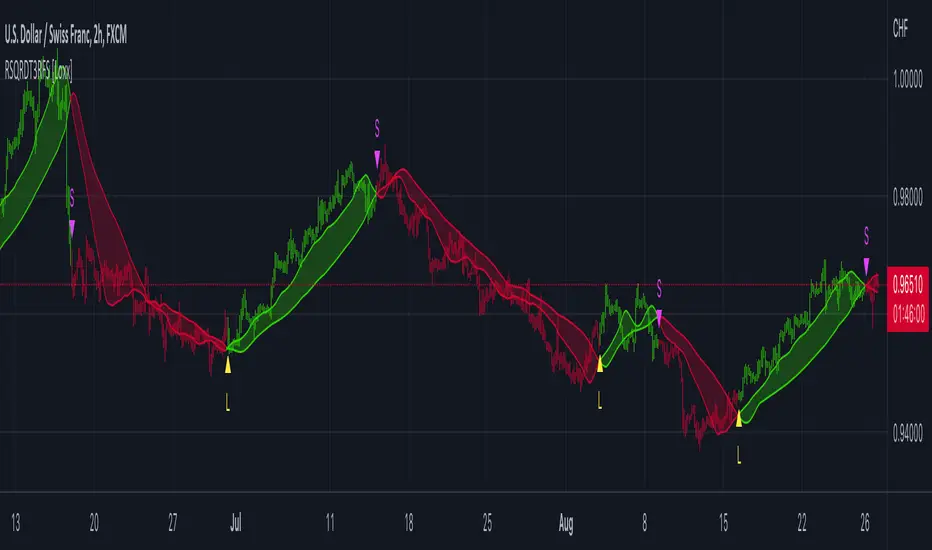
T3 Slope Variation [Loxx]T3 Slope Variation is an indicator that uses T3 moving average to calculate a slope that is then weighted to derive a signal.
The center line
The center line changes color depending on the value of the:
Slope
Signal line
Threshold
If the value is above a signal line (it is not visible on the chart) and the threshold is greater than the required, then the main trend becomes up. And reversed for the trend down.
Colors and style of the histogram
The colors and style of the histogram will be drawn if the value is at the right side, if the above described trend "agrees" with the value (above is green or below zero is red) and if the High is higher than the previous High or Low is lower than the previous low, then the according type of histogram is drawn.
What is the T3 moving average?
Better Moving Averages Tim Tillson
November 1, 1998
Tim Tillson is a software project manager at Hewlett-Packard, with degrees in Mathematics and Computer Science. He has privately traded options and equities for 15 years.
Introduction
"Digital filtering includes the process of smoothing, predicting, differentiating, integrating, separation of signals, and removal of noise from a signal. Thus many people who do such things are actually using digital filters without realizing that they are; being unacquainted with the theory, they neither understand what they have done nor the possibilities of what they might have done."
This quote from R. W. Hamming applies to the vast majority of indicators in technical analysis . Moving averages, be they simple, weighted, or exponential, are lowpass filters; low frequency components in the signal pass through with little attenuation, while high frequencies are severely reduced.
"Oscillator" type indicators (such as MACD , Momentum, Relative Strength Index ) are another type of digital filter called a differentiator.
Tushar Chande has observed that many popular oscillators are highly correlated, which is sensible because they are trying to measure the rate of change of the underlying time series, i.e., are trying to be the first and second derivatives we all learned about in Calculus.
We use moving averages (lowpass filters) in technical analysis to remove the random noise from a time series, to discern the underlying trend or to determine prices at which we will take action. A perfect moving average would have two attributes:
It would be smooth, not sensitive to random noise in the underlying time series. Another way of saying this is that its derivative would not spuriously alternate between positive and negative values.
It would not lag behind the time series it is computed from. Lag, of course, produces late buy or sell signals that kill profits.
The only way one can compute a perfect moving average is to have knowledge of the future, and if we had that, we would buy one lottery ticket a week rather than trade!
Having said this, we can still improve on the conventional simple, weighted, or exponential moving averages. Here's how:
Two Interesting Moving Averages
We will examine two benchmark moving averages based on Linear Regression analysis.
In both cases, a Linear Regression line of length n is fitted to price data.
I call the first moving average ILRS, which stands for Integral of Linear Regression Slope. One simply integrates the slope of a linear regression line as it is successively fitted in a moving window of length n across the data, with the constant of integration being a simple moving average of the first n points. Put another way, the derivative of ILRS is the linear regression slope. Note that ILRS is not the same as a SMA ( simple moving average ) of length n, which is actually the midpoint of the linear regression line as it moves across the data.
We can measure the lag of moving averages with respect to a linear trend by computing how they behave when the input is a line with unit slope. Both SMA (n) and ILRS(n) have lag of n/2, but ILRS is much smoother than SMA .
Our second benchmark moving average is well known, called EPMA or End Point Moving Average. It is the endpoint of the linear regression line of length n as it is fitted across the data. EPMA hugs the data more closely than a simple or exponential moving average of the same length. The price we pay for this is that it is much noisier (less smooth) than ILRS, and it also has the annoying property that it overshoots the data when linear trends are present.
However, EPMA has a lag of 0 with respect to linear input! This makes sense because a linear regression line will fit linear input perfectly, and the endpoint of the LR line will be on the input line.
These two moving averages frame the tradeoffs that we are facing. On one extreme we have ILRS, which is very smooth and has considerable phase lag. EPMA has 0 phase lag, but is too noisy and overshoots. We would like to construct a better moving average which is as smooth as ILRS, but runs closer to where EPMA lies, without the overshoot.
A easy way to attempt this is to split the difference, i.e. use (ILRS(n)+EPMA(n))/2. This will give us a moving average (call it IE /2) which runs in between the two, has phase lag of n/4 but still inherits considerable noise from EPMA. IE /2 is inspirational, however. Can we build something that is comparable, but smoother? Figure 1 shows ILRS, EPMA, and IE /2.
Filter Techniques
Any thoughtful student of filter theory (or resolute experimenter) will have noticed that you can improve the smoothness of a filter by running it through itself multiple times, at the cost of increasing phase lag.
There is a complementary technique (called twicing by J.W. Tukey) which can be used to improve phase lag. If L stands for the operation of running data through a low pass filter, then twicing can be described by:
L' = L(time series) + L(time series - L(time series))
That is, we add a moving average of the difference between the input and the moving average to the moving average. This is algebraically equivalent to:
2L-L(L)
This is the Double Exponential Moving Average or DEMA , popularized by Patrick Mulloy in TASAC (January/February 1994).
In our taxonomy, DEMA has some phase lag (although it exponentially approaches 0) and is somewhat noisy, comparable to IE /2 indicator.
We will use these two techniques to construct our better moving average, after we explore the first one a little more closely.
Fixing Overshoot
An n-day EMA has smoothing constant alpha=2/(n+1) and a lag of (n-1)/2.
Thus EMA (3) has lag 1, and EMA (11) has lag 5. Figure 2 shows that, if I am willing to incur 5 days of lag, I get a smoother moving average if I run EMA (3) through itself 5 times than if I just take EMA (11) once.
This suggests that if EPMA and DEMA have 0 or low lag, why not run fast versions (eg DEMA (3)) through themselves many times to achieve a smooth result? The problem is that multiple runs though these filters increase their tendency to overshoot the data, giving an unusable result. This is because the amplitude response of DEMA and EPMA is greater than 1 at certain frequencies, giving a gain of much greater than 1 at these frequencies when run though themselves multiple times. Figure 3 shows DEMA (7) and EPMA(7) run through themselves 3 times. DEMA^3 has serious overshoot, and EPMA^3 is terrible.
The solution to the overshoot problem is to recall what we are doing with twicing:
DEMA (n) = EMA (n) + EMA (time series - EMA (n))
The second term is adding, in effect, a smooth version of the derivative to the EMA to achieve DEMA . The derivative term determines how hot the moving average's response to linear trends will be. We need to simply turn down the volume to achieve our basic building block:
EMA (n) + EMA (time series - EMA (n))*.7;
This is algebraically the same as:
EMA (n)*1.7-EMA( EMA (n))*.7;
I have chosen .7 as my volume factor, but the general formula (which I call "Generalized Dema") is:
GD (n,v) = EMA (n)*(1+v)-EMA( EMA (n))*v,
Where v ranges between 0 and 1. When v=0, GD is just an EMA , and when v=1, GD is DEMA . In between, GD is a cooler DEMA . By using a value for v less than 1 (I like .7), we cure the multiple DEMA overshoot problem, at the cost of accepting some additional phase delay. Now we can run GD through itself multiple times to define a new, smoother moving average T3 that does not overshoot the data:
T3(n) = GD ( GD ( GD (n)))
In filter theory parlance, T3 is a six-pole non-linear Kalman filter. Kalman filters are ones which use the error (in this case (time series - EMA (n)) to correct themselves. In Technical Analysis , these are called Adaptive Moving Averages; they track the time series more aggressively when it is making large moves.
Included
Alets
Signals
Bar coloring
Loxx's Expanded Source Types